CUPED
Experiment setup
goal is to estimate the delta = mean(Y_c) - mean(Y_t)
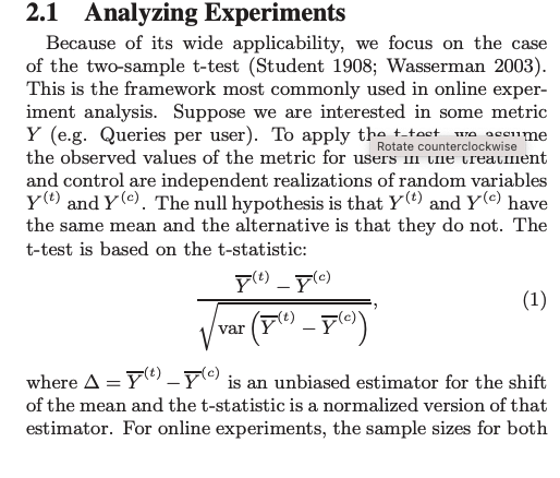
We want this estimate to have small varaince and to be unbiased.
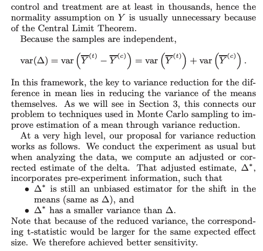
In this framework, the key to variance reduction for the difference in mean lies in reducing the variance of the means themselves.
What is CUPED?
CUPED is a well-established variance reduction technique for experiments paper
Unlike methods like outlier removal or winsorization, it doesn’t sacrifice any data integrity.
It can be used together with winsorization, which enhances its effectiveness.
It requires pre-experimentation data - which we generally have in Bunsen.
For a rather unpredictable event like ad clicks, we get ~5% reduction in standard deviation (which is ~10% reduction in variance, and experiment run time). For something like sessions, that 5% can increase to something like 30%.
Predicted uncertainty is not uncertainty.
So the variance in your experiment metric should only take into account the unpredictable part of your measurement. If you predict that:
- guv A will have 5 sessions during the experiment, and
- guv B will have 20 sessions,
And when you actually measure the sessions, you get:
- guv A has 4 sessions (-1 from prediction)
- guv B has 21 sessions (+1 from prediction),
Then the variance, or the uncertainty, in your measurement can be calculated on the residuals of your predictions, rather than on the measurements themselves. This gives var([-1, +1]), rather than var([4, 21]), which is a great reduction.
Control Variates
From paper:
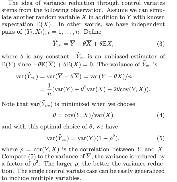
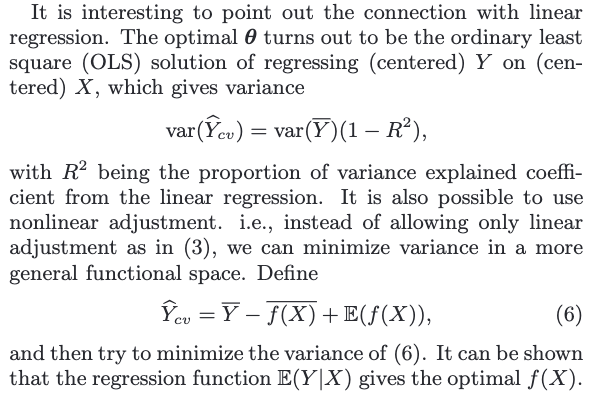
Control Variates in online experiments
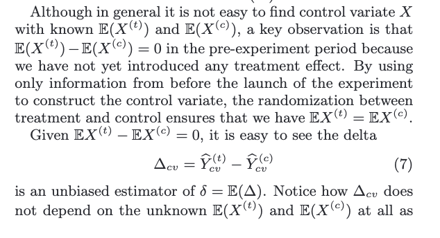
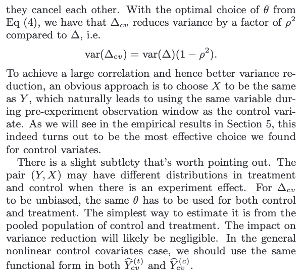
The difficulty of applying it boils down to finding a control variate that is highly correlated with and at the same time has known .
cv stands for control varaites
Control Variates vs Stratification
See Stratification
These are two techniques that both utilize covariates to achieve variance reduction. The stratification approach uses the covariates to construct strata while the control variates approach uses them as regression variables.
The former uses discrete (or discretized) covariates, whereas control variates seem more naturally to be continuous variables.
Control Variates is an extension of stratification, where the covariate can be an indicator variable showing the belonging of a sample to a stratum.
While these two techniques are well connected mathematically, they provide different insights into understanding why and how to achieve variance reduction. The stratification formulation has a nice analogy with mixture models, where each stratum is one component of the mixture model. Stratification is equivalent to separating samples according to their component memberships, effectively removing the between-component variance and achieving a reduced variance. A better covariate is hence the one that can better classify the samples and align with their underlying structure. On the other hand, the control variates formulation quantifies the amount of variance reduction as a function of the correlation between the covariates and the variable itself. It is mathematically simpler and more elegant. Clearly, a better covariate should be the one with larger (absolute) correlation.
CUPED IN PRACTICE
A simple yet effective way to implement CUPED is to use the same variable from the pre-experiment period as the covariate. You need to have pre-experiment data (have not applied treatment), not good when you work with new users.
The more correlated covariate with the target the larger variance reduction.
Across a large class of metrics, our results consistently showed that using the same variable from the pre-experiment period as the covariate tends to give the best variance reduction. In addition, the lengths of the pre-experiment and the experiment periods also play a role. Given the same pre-experiment period, extending the length of the experiment does not necessarily improve the variance reduction rate. On the other hand, a longer pre-period tends to give a higher reduction for the same experiment period.
- margarida's implementation
-- winsorization 90th %tile + CUPED

  WITH bucketed_assignment_log AS (
      -- macro assign_cohorts start
      SELECT cohort_id,
             user_id_encid,
             MIN(first_assignment_time) - INTERVAL '5 SECOND' AS first_assignment_time
        FROM dl_bunsen_filtered.assignment_log_metric_analysis_v2
       WHERE experiment_run_id = 11052
         AND (is_bot = FALSE OR is_bot IS NULL)
         AND first_assignment_time BETWEEN '2023-07-25' -- wildcards are timestamp strings, e.g. '2022-07-28 12:00:00'
           AND '2023-09-25' -- note that the single quotes are required
       GROUP BY 1, 2
      -- macro assign_cohorts end
  ),

       connections_data AS (SELECT connections.user_id_encid,
                                   connections.object_id,
                                   datapipe_timestamp AS event_time
                              FROM dl_bunsen_mad.connections_sessionized_bot_labeled AS connections
                             WHERE TIMESTAMP 'epoch' + datapipe_event_time / 1000000 * INTERVAL '1 second' BETWEEN '2023-07-25'
                                 AND '2023-09-25'
                               AND connections.dt BETWEEN (DATE_TRUNC('day', '2023-07-25'::TIMESTAMP) - INTERVAL '1 DAY')
                                 AND (DATE_TRUNC('day', '2023-09-25'::TIMESTAMP) + INTERVAL '1 DAY')
                               AND connection_type IN ('photo_uploaded')
                               AND is_bot = 'false'
                             GROUP BY 1, 2, 3),

       sum_per_day_per_user AS (SELECT cohort_id,
                                       bucketed_assignment_log.user_id_encid,
                                       first_assignment_time,
                                       COUNT(DISTINCT object_id) AS sum_per_day_per_user
                                  FROM bucketed_assignment_log
                                  INNER JOIN connections_data
                                      ON bucketed_assignment_log.user_id_encid = connections_data.user_id_encid
                                          AND
                                         connections_data.event_time BETWEEN bucketed_assignment_log.first_assignment_time
                                             AND '2023-09-25'
                                 GROUP BY 1, 2, 3),

       percentile_reviews AS (SELECT user_id_encid,
                                     sum_per_day_per_user,
                                     PERCENTILE_CONT(0.90) WITHIN GROUP (ORDER BY sum_per_day_per_user)
                                     OVER () AS percentile_90
                                FROM sum_per_day_per_user),

       censored_photos AS (SELECT user_id_encid,
                                  CASE
                                      WHEN sum_per_day_per_user <= percentile_90 THEN sum_per_day_per_user
                                      ELSE percentile_90
                                      END AS photos_censored
                             FROM percentile_reviews),

       sum_per_user AS (SELECT cohort_id,
                               user_id_encid,
                               first_assignment_time,
                               COALESCE(photos_censored, 0) /
                               (DATEDIFF(SEC,
                                         TO_DATE('2023-07-25', 'YYYY-MM-DD'),
                                         TO_DATE('2023-09-25', 'YYYY-MM-DD')) / 86400.
                                   )::FLOAT AS avg_sum_per_user
                          FROM bucketed_assignment_log
                          LEFT JOIN censored_photos
                              USING (user_id_encid)),

       get_theta AS (SELECT cohort_id,
                            user_id_encid,
                            X,
                            Y,
                            avg_X,
                            avg_Y,
                            var_X,
                            SUM((X - avg_X) * (Y - avg_Y) / (N - 1)) OVER () AS cov_XY,
                            cov_XY / var_X                                   AS theta
                       FROM (SELECT cohort_id,
                                    sum_per_user.user_id_encid,
                                    COALESCE(num_photos_in_last_year, 0) AS X,
                                    avg_sum_per_user                     AS Y,
                                    COUNT(*) OVER ()                     AS N,
                                    AVG(X) OVER ()                       AS avg_X,
                                    AVG(Y) OVER ()                       AS avg_Y,
                                    VARIANCE(X) OVER ()                  AS var_X
                               FROM sum_per_user
                               LEFT JOIN data_science.contribution_summary
                                   ON sum_per_user.user_id_encid = contribution_summary.user_id_encid
                                       AND contribution_summary.dt =
                                           (SELECT MAX(dt) FROM data_science.contribution_summary)) AS aux
                      GROUP BY cohort_id,
                               user_id_encid,
                               X,
                               Y,
                               avg_X,
                               var_X,
                               avg_Y,
                               N),

       get_Y_cuped AS (SELECT cohort_id,
                              user_id_encid,
                              Y - theta * (X - avg_X) AS Y_cuped
                         FROM get_theta
                        GROUP BY cohort_id,
                                 user_id_encid,
                                 X,
                                 Y,
                                 avg_X,
                                 theta)

SELECT cohort_id,
       COUNT(user_id_encid) AS sample_size,
       AVG(Y_cuped)         AS metric_value,
       STDDEV(Y_cuped)      AS standard_deviation
  FROM get_Y_cuped
 GROUP BY cohort_id
 ORDER BY cohort_id;