Design and Analysis of Algorithms
MIT 6.046
Lecture notes. All notes + your marks in one place here
Lecture videos
Overview of course:
- Divide and Conquer (Merge Sort classic example, Fast Fourier transform, algorithm for convex hull, van Emde Boas trees)
- Amortized analysis, random algos, quick select,quick sort skip lists, perfect and universal hashing
- Optimization (greedy (Dijkstra), dynamic programming, shortest paths)
- Network Flow (network, capacities, max flow - min cut problem)
- Linear Programming
- Intractability (polynomial vs exponential time problems, approximation problems)
- Synchronous, Asynchronous algos, Cryptography, RSA
- Cache, External Memory Model, Cache Oblivious Model, Complexity in terms of memory transfers
Lecture 1. Interval Scheduling
Very similar problems can have very different complexity. Wiki problem definition.
Polynomial: Shortest path between two vertices. O(V**2)
NP: Determine if a graph has Hamiltonian cycle: Given a directed graph find a simple cycle that contain each vertex V.
NP-complete are the hardest problems in NP. Solve a NP-complete in polynomial time, then you can solve all NP problems.
Given an array of intervals [(s1,f1), (s2,f2) ... ] - left closed, right opened. Select the maximum number of non-overlapping intervals.
This problem should not be confused with meeting rooms problem where we find minimum
conference rooms needed (time with max overlap). The latter is line sweep.
Claim We can solve this problem using a greedy algorithm.
Definition A greedy algorithm is a myopic algorithm that processes the input one piece at a time with no apparent look ahead.
Non-working greedy heuristics:
- pick shortest intervals
- pick intervals with least amount of overlaps. Counter example:
---- ---- ---- ----
  ----- ---- ----
  -----      ----
  -----      ----
  -----      ----
Working greedy heuristic:
- pick earliest finish time
"Proof by intimidation, proof because the lecturer said so"
Proof by induction
Claim: Given a list of intervals L, greedy algorithm with earliest finish time produces k* intervals, where k* is maximum
Induction on k*! Induction on the number of optimal intervals.
- Base case
k* = 1. Any interval can be picked up. - Suppose claim holds for
k*and we are given a list of intervals whose optimal schedule hask*+1intervals
Run our greedy algo and get intervals . and are not comparable, yet. By construction . Thus is another optimal solution of size . Let be the set of intervals where . is optimal for then is optimal solution of and has size . By initial hypothesis we run greedy on and produce of size . Then and proves the when we run greedy and get is also optimal solution.
Problem. Weighted interval scheduling. Each interval has a weight . Find a schedule with maximum total weight.
Greedy does not work here, need to use DP
- subproblem space:jobs[i:], dp(i) is max profit given jobs[i:]
- need NOT neccessarily include job[i]
- note need to sort by start/end time
- need to sort by start time and define subproblem jobs[i:] or sort by end time and define subproblem to be s[:i]
- O(n**2) is easy
- improve to O(nlogn) with BS
`
CODE
# O(n^2)
class Solution:
    def jobScheduling(self, start: List[int], end: List[int], profit: List[int]) -> int:
        @cache
        def dp(i):
            if i == len(jobs): return 0
            val = max(dp(i+1),jobs[i][2])
            for j in range(i+1,len(jobs)):
                if jobs[i][1] <= jobs[j][0]:
                    val = max(val,dp(j)+jobs[i][2])
            return val
        jobs = [(s,e,p) for s,e,p in zip(start,end,profit)]
        jobs.sort(key=lambda x:x[0])
        return dp(0)

# O(nlog(n))
class Solution:
    def jobScheduling(self, start: List[int], end: List[int], profit: List[int]) -> int:
        def bs(l,r,num):
            while l<r:
                m = l+r>>1
                if jobs[m][0]>=num:
                    r = m
                else:
                    l = m+1
            return l
        @cache
        def dp(i):
            if i == len(jobs): return 0
            j = bs(i+1,len(jobs),jobs[i][1])
            return max(dp(i+1),dp(j)+jobs[i][2])
        jobs = [(s,e,p) for s,e,p in zip(start,end,profit)]
        jobs.sort(key=lambda x:x[0])
        return dp(0)

# O(nlog(n))
class Solution:
    def jobScheduling(self, start: List[int], end: List[int], profit: List[int]) -> int:
        def bs(l,r,num):
            while l<r:
                m = l+r>>1
                if jobs[m][1]>num:
                    r=m
                else:
                    l=m+1
            return l-1
        @cache
        def dp(j):
            if j < 0: return 0
            i = bs(0,j,jobs[j][0])
            return max(dp(j-1),dp(i)+jobs[j][2])

        jobs = [(s,e,p) for s,e,p in zip(start,end,profit)]
        jobs.sort(key=lambda x:x[1])
        return dp(len(jobs)-1)
NP-complete problem. Generalization of the problem considers machines/resources.Here the goal is to find compatible subsets whose union is the largest. First example had k = 1.
In an upgraded version of the problem, the intervals are partitioned into groups. A subset of intervals is compatible if no two intervals overlap.
Lecture 2. Divide & Conquer: Convex Hull, Median Finding
Divide and Conquer Paradigm: Given a problem of size :
- Divide it into subproblems of size where so that your subproblems have smaller size.
- Solve each subproblem recursively
- Combine solutions of subproblems into overall solution (this is where the smarts of the algo is).
Run-time: . Often to compute you can use Master Theorem.
Convex Hull Problem
Given points in a plane assume no two have the same coordinate and no two have the same coordinate and no three line on the same line. The convex hull is the smallest polygon which contains all points in .
Simple algorithm:
- For each pair of points draw a line.
- This line separates the plane in two half-planes.
- Check if all points lie in one side on the half-plane. If yes, this line is part of the convex hull (we call it a segment of the convex hull), otherwise it is not a segment.
Run-time: pairs of points, to test runtime.
Divide and Conquer algo:
- Sort the points by x coordinates.
- For input set , divide into left half and right half by coordinates.
- Compute convex hull for and for .
- Combine solutions.
Obvious algorithm looks at all pairs and takes runtime
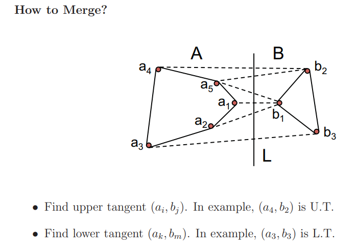
Find upper, and lower tangent using two finger and a string algorithm. Compute intercept of the vertical line and all points. Algo demo.
Merge step: After you find the tangents and you link to go down all till you see , then link to then go up through all till you see .
Run time
Other Convex Hull solutions:
- dbabichev chain multiplication?
Median Finding Algorithm
It is just quick-select algo. Randomized pivot point has expected run time and worse case. Smart pivot point is a deterministic algo (groups of 5 elements, median of medians) has worse case time. See CLRS for detailed algo (deterministic) time to find median.
Lecture 3. Divide & Conquer: Fast Fourier Transform
Polynomial of order
Operations on polynomial:
- evaluation . Use Horner's rule to do it in . - multiplications and additions
- addition
- multiplication , The coefficients of are and that takes time, so in total brute force multiplication of polynomials takes run time.
Polynomial multiplication is the same as doing convolution between vectors.
u = [1 1 1];
v =  [1 1 0 0 0 1 1];
1  1  1 -> 1
   1  1 1 -> 2
      1 1 1 -> 2
conv(u,v) =  [1     2     2     1     0     1     2     2     1]
moves as a filter through . Think convolutional neural networks! In polynomial multiplication
Polynomial representation
- coefficient vector =
- roots (allowing multiplicity).
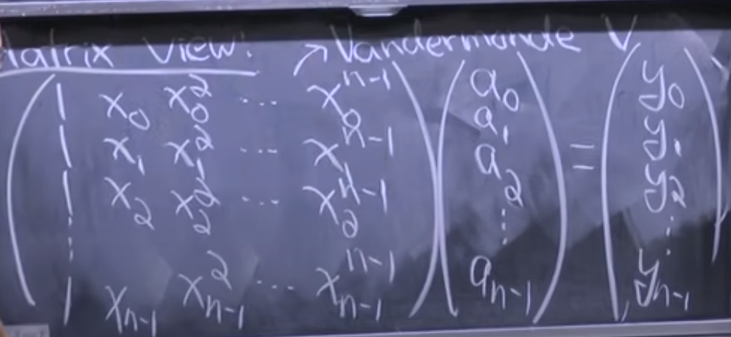
- samples/points (x_k,y_k) for for has unique solution by the Fundamental Theorem in Algebra
By FTA allowing multiplicity define uniquely the polynomial.
root representation is not good. Hard to go from polynomial to root representation. Addition is also very hard. Multiplication is easy.
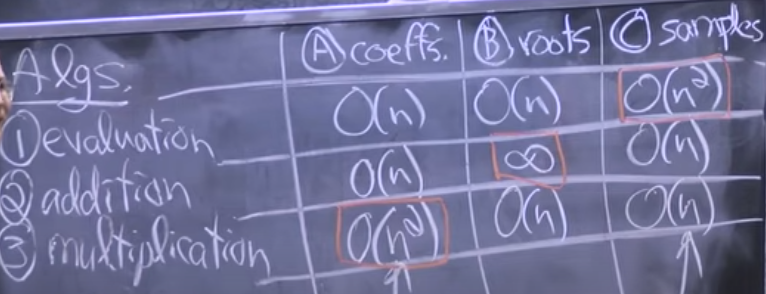
No representation is perfect! Our aim is to convert from coefficient to sample representation in time using Fourier transform.
Coefficient repr -> Samples repr can be done in trivially
- gets you the sample representation on
- Samples to coefficients ( and are known how would you find ):
- Gaussian elimination
- Multiply by inverse - computing inverse once and use for free.
Divide & Conquer Algorithm
We have coefficient representation and want to get samples in time.
- Divide into even and odd coefficients.
-
Conquer: Recursively compute and for
-
Combine:
Run time
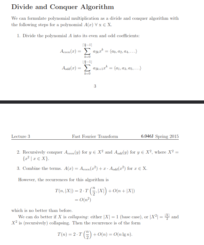
To get collapsing set :
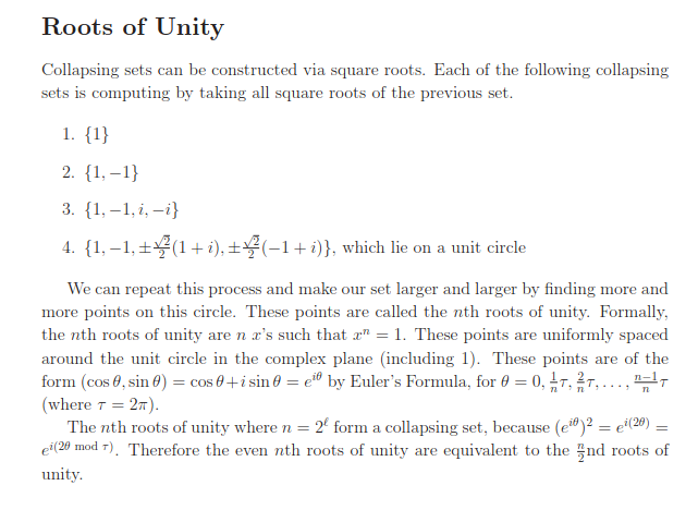
dbabichev FFT implementation.
np.convolve is much slower as it does not use FFT. scipy has convolve function and uses FFT.
Lecture 4. Divide & Conquer: van Emde Boas Trees
Emde Boas Tree.
Goal: Maintain elements among subject to insert, delete, successor (given a value I want to know the next greater value in the set). We know how to do all these in time using balance BST-s (AVL, Red-Black). Emde Boas Trees can doo these in which is an exponential improvement.
Intuition: Binary search on the levels of the tree where the number of levels is
Can we do better than and does not depend on the universe of numbers ? No.
In each of previous tree data structures, where we do stuff dynamically, at least one important operation took time, either worst case or amortized. In fact, because each of these data structures bases its decisions on comparing keys, the lower bound for sorting tells us that at least one operation will have to take time. Why? If we could perform both the INSERT and EXTRACT-MIN operations in o.lg n/ time, then we could sort keys in time by first performing INSERT operations, followed by EXTRACT-MIN operations.
First attempt to store an array of size with elements among the set :
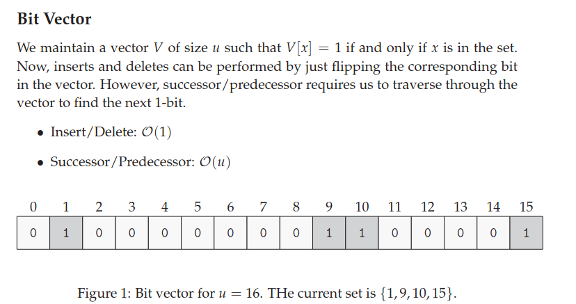
Insert and Delete are constant, Successor is linear.
Second attempt:
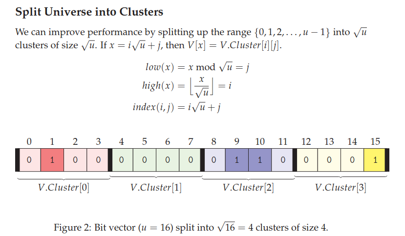
Think each cluster as a binary tree built bottom up using the OR operation. All roots of the different clusters will be a 'summary' vector. As this vector will tell you if there is a one in each of the clusters.
Insert is constant - need to change the value in the clusters and mark in the summary vector.
Successor is:
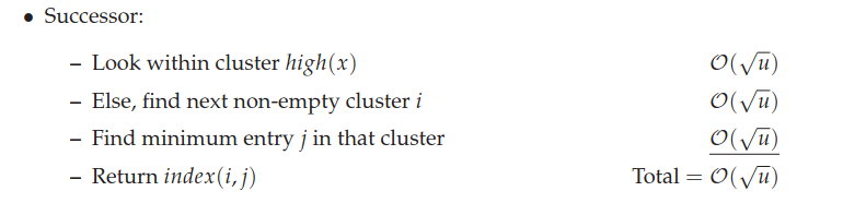
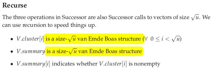
We have not yet improved the runtime complexity. Van Emde Boas is to create clusters which are recursive and depend on other clusters.
Code implementation details look at the lecture and your notes here.
Lecture 5: Amortization
So far learning fancy cool data structures. This lecture is on fancy cool techniques of computing complexity of data structures.
Amortized analysis is used to compute complexity of data structures. It computes the total run time of a data structure given executed operations. Amortized analysis is not used in computing run time of algorithms.
Table doubling
That's how dynamic arrays work in Python.
Assume a table of size . We will double the size of the table whenever it is full. For insertions the total running time is:
. Thus amortized (i.e.) per insertion it is .
Techniques of amortized analysis:
- aggregate method
- accounting method
- potential method
All these method give upper bounds to the actual cost of all operations = amortized cost.
Aggregate method
This is what we did in table doubling. Added total cost of operations then divided by . NB: Often when you have a data structure with total of insert and delete operations you can just think of insert operations because each element can be deleted at most the number of times it has been inserted.
Accounting method
Store credit bank account which should always be non-negative. When you do an operation you pay for the operation and can deposit money in you account.
Example. Table Doubling.
-
If insertion does not trigger table doubling: I would pay 1 coin for the insertion plus c coin deposit.
-
If insertion trigger table doubling: I can pay from the bank account to cover the table doubling.
-
amortized cost for table doubling when the table becomes of size is for chosen large enough . When table doubles from to , only last places have coins.
-
amortized runtime per insertion
Aside. Table expansion and contraction have insert and delete operations in amortized if:
- table doubling when table is full
- table contraction by a halve when there are elements in the table of size
To prove this is indeed amortized you need the Potential method.
Potential method
Define a potential (energy) function which maps each data structure to a nonnegative integer. Check CLRS for more details and proof of Table doubling and halving is .
Lecture 6: Randomized Algorithms
Randomized algorithm is one that generates a random number and makes decisions on 's value.
On same input and on different execution randomized algos may:
- run a different number of steps
- produce different output
Two types of random algos:
- Monte Carlo - runs in polynomial time always output is correct with high probability
- Las Vegas - runs in expected polynomial time output is always correct
Monte Carlo = probably correct Las Vegas = probably fast
Monte Carlo is for estimation stuff to get almost correct values.
Las Vegas example is quick sort - expected time. 'Almost sorted' does not make sense.
Problem. Matrix Product Checker
Given n$ matrices the goal is to check if x . We use randomized algo so that we do not checkout the full multiplication.
Freivalds' algorithm
Procedure:
- Generate an random vector .
- Compute
- Output "Yes" if ; "No," otherwise.
If , then the algorithm always returns "Yes". If then the probability that the algorithm returns "Yes" is less than or equal to one half.
By iterating the algorithm times and returning "Yes" only if all iterations yield "Yes", a runtime of and error probability of is achieved.
Proof that false negatives. Idea is for every bad which does not catch that we create a good and have 1-1 mapping. See your notes.
Paranoid Quick Sort
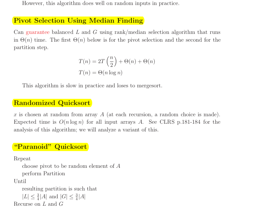
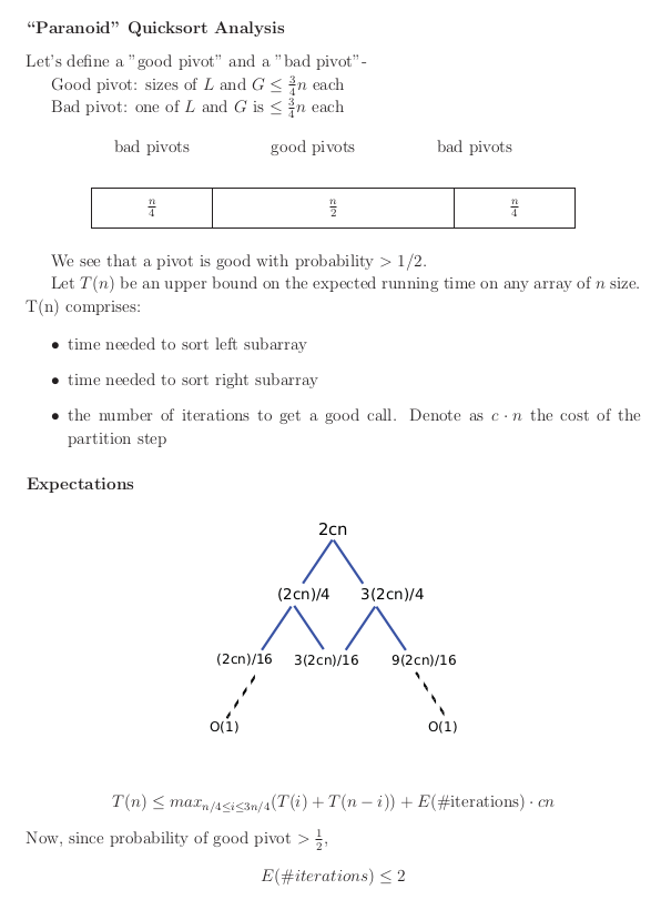
Paranoid Quick sort is probably fast with expected running time .
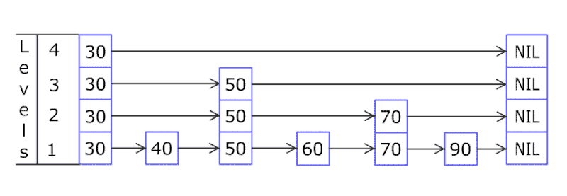
Lecture 7 Randomization: Skip Lists
A skip list a probabilistic data structure that allows search, insert, delete within a set of elements. It maintains a linked list hierarchy of subsequences with each successive subsequence skipping over fewer elements than the previous one. In the example below we insert 80.
Comparing with treap and red-black tree which has the same function and performance, the code length of Skiplist can be comparatively short and the idea behind Skiplists is just simple linked lists.
Design a skip list, leetcode.
Motivation for skip lists.
Step 1. Linked list - search is
Step 2. Sorted Linked list - search is still
Step 3. Two sorted Linked list, where the second one is a subsequence (express line) and skips elements.
Step 4. Add layers of linked lists
- Insert is randomized using a fair coin
- Search and Delete are deterministic
Why skip lists are good?
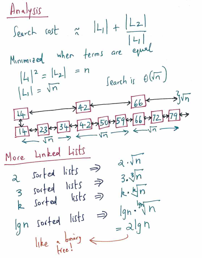
Warm-up Lemma, The number of levels in element skip list is with high probability, that is as grows we the probability converges to 1. This is stronger than having expected running times stuff where you have no guarantees of how likely the worst case is.
With this lemma we can say thing like:
- number of levels in the skip list is at most with probability
- at most with probability etc
Proof. some element got promotions
Search
Theorem. Any search in -element skip list costs
Steps:
- We track the search moves backwards
- Backwards search makes up and left moves each with probability 1/2
- Number of ups is less than number of levels with high probability
- The BUM: Total number of moves = number of coin flips until you get heads (up moves)
Claim: Number of coin flips until we see heads is with high probability.
We need to proof that for to see heads, there exist a constant such that if is a random vairable counting the number of heads after coin flips then . Idea is to use Chernoff bound.
Lecture 8: Randomization: Universal & Perfect Hashing
Buzz words: Hashing with chaining, open addressing, load factor , Simple Uniform Hashing assumption, Hash functions, linear probing, quadratic probing, universal hashing, perfect hashing
Dictionary problem. Abstract Data Type (Math definition, interface):
- maintain a dynamic set of items
- each item has a key, item is a key value pair
- insert(item)
- delete(item)
- search(key)
Goal is to run all 3 operations in expected time (amortized).
In MIT 6.001- Introduction to Algorithms you saw hashing with chaining and open addressing. you proved that the insert, delete and search take , where n is the number of elements you have in the table and m is the number of slots (table size, number of buckets). So as long as you chose (you can keep that dynamically using table doubling and shrinking) you would have operations.
However, you assumed that you have simple uniform hashing. That is your keys are mapped at each slot of the table with probability So you had to choose a smart hashing function that would map your keys uniformly. However you want, a hashing function that work work well no matter what the keys are. That is in the worst case scenario for the keys you still want operations. Our analysis in MIT 6.001 considered average case scenario, where for random keys we would have simple uniform hashing.
Want to avoid the assumption that the keys are random.
Universal Hashing
Works for dynamic sets - allows insert and delete
- choose randomly from a hash family .
- assume ti be universal hash family:
- for all keys : , probability over choosing .
You can prove using indicator variables that number of keys hashing to the same place as
Dot product hash family
- assume m is prime
- assume for integer
- view key in base ,
- for a key define (dot product)
. To choose random choose a random .
Another universal hashing family:
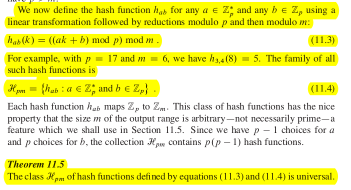
We achieved expected time for all operations.
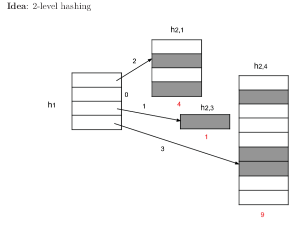
Perfect Hashing
This works for static keys and support search only. It is perfect hashing because it achieves search worst case, that is keys are stored perfectly with no collisions.
- polynomial build time with high probability
- worst case run time
- worst case memory
Idea: Use 2-level hashing.
Lecture 9: Augmentation. Range Trees
Easy Tree Augmentation.
The goal here is to store at each node , which is a function of the node, namely subtree rooted at . If is computable locally from its children then updates take runtime where h is the height of the tree. To update , we need to walk up the tree to the root.
Order-statistic trees.
ADT (interface of the data structure):
- insert(x), delete(x), successor(x)
- rank(x)
- select(i): find me the element of rank i
Want all of these in
We can implement the above ADT using easy tree augmentation on AVL trees (or 2-3 trees or any balance BST) to store subtree size: subtree = # of nodes in it.
![]()
NB: Need to choose augmentation functions which can be maintained easier such as subtree size. Above we could thing to store the rank of each node (rank and select would be very easy). However if you insert elements it would be , e.g. if you insert a minimum element you need to update all node ranks.
#TODO Finger Search Trees (this is tree augmentation on 2-3 threes)
Range Trees
Solves the problem orthogonal range search.
Suppose we have points in a -dimension space. We would like a data structure that supports range query on these points: find all the points in a give axis-aligned box. An axis-aligned box is simply an interval in 1D, a rectangle in 2D, and a cube in 3D.
Goal is to run in output size .
NB: Our data structure would be static and support only search points in box query.
1D case
We have array [a_1,a_2...a_n] and for a query search(x,y) we want to output all numbers in the array which are in the interval [x,y). Simple solution is to use sorted array and then do binary searches in .
Sorted arrays are inefficient for insertion and deletion. For a dynamic data structure that supports range queries such as AVL, Red-Black trees.
However, neither of the above approaches generalizes to high dimensions.
1D range trees
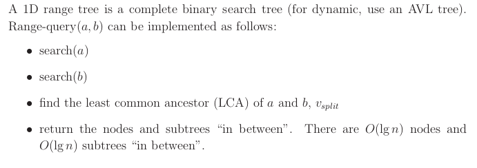
That is like doing rightful rank for node and left rank for node .
Analysis. to implicitly represent the answer (showing just the roots). to output all k answers. to report k via subtree size augmentation.
2D range trees
Create a 1D range tree on the x coordinates. Do a search to find nodes which satisfy the interval provided by the coordinate. Data Augmentation: for each of these trees we store another range tree on the y coordinate. So we have dictionary with keys being the nodes of the first range tree, and values is range tree by the y coordinate. There is lots of data duplication. Then you do a little search on the . Run time
Space complexity is . The primary subtree is . Each point is duplicated up to times in secondary subtrees, one per ancestor.
Aside
Range trees are used in database searches. For example if you have 4 columns in a database and you do searches like col1 should be inside one interval col2 in another interval, etc. range trees would allow fast queries. This is called indexing in database columns.
Lecture 10: Dynamic Programming. Advanced DP
We consider 3 problems:
- longest palindromic subsequence
- optimal binary search tree
- alternating coin game
DP steps:
- Determine Subspace of problems
- Define Recursive relation based on optimal solutions of subproblem
- Compute value of an optimal solution (bottom-up, top down)
- Construct optimal solution from computed information (typically involves some backtracing)
Longest Palindromic Sequence Given a string find the longest subsequence which is a palindrome (not necessarily contiguous).
Solution `
CODE
# O(n**2)
def solve(s):
    @cache
    def dp(i,j):
      if i == j: return 1
      elif  i > j: return 0
      if s[i] == s[j]: return 2 + dp(i+1,j-1)
      return max(dp(i+1,j),dp(i,j-1))
Run time = Number of subproblems * Time per subproblem (assumes lookup is )
If you use arrays for lookup you would have constant access, in hash tables you get it constant amortized (collisions).
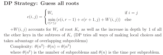
Optimal Binary Search Trees
Given keys , where WLOG . There are many different BST-s with these set of keys. We assign weights for each of these keys . You can think that the weights are probabilities of searching each of the keys (search probabilities). Find/construct a BST that minimizes:
depth .
The root has depth 0. Application: needs a structure which would minimize the expected search cost.
Before doing DP, try greedy!
We choose the root to be the key with largest weight. Then you know which nodes are on the left and which on the right. Continue do greedy approach in recursive fashion. But this does not work:
DP solution
Subproblem space cost of optimal BST on
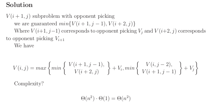
Alternating Coin Gamse
Row of coins of values , where is even. In each turn, a player selects either the first or last coin from the row, removes it, and receives the value of the coin
The first player never looses (win or equal)! He can make it so that he pick all values on odd indices or on even indices, depending which sum gives the larger sum.
How to maximize the amount of money won assuming you move first?
Subproblem space: is the max value we can definitely win if it is our turn and only conis
Lecture 11. Dynamic Programming. All-Pairs Shortest Paths
Two types of shortest path problems:
- single source (from one source find the shortest path to all vertices )
- all pairs shortest path
The problem with one source and one destination cannot be solved faster than the single source shortest path, so when you solve it you would use the single source shortest path solutions such as Dijkstra and Bellman Ford.
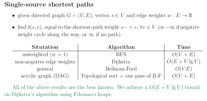
Note that Dijkstra works only for non-negative weights. It is a type of greedy algorithm.
Bellman Ford works for general graphs. It is a DP algo.
APSP = All pairs shortest path
One way to solve this problem is to run times Dijkstra or Bellman Ford.
DP First attempt.
If your subproblem space is that is shortest path from to , then you would not have a DAG subproblem space! Enter an infinite recursion when trying to resolve your subproblems.
Natural improvement of subspace is dp[u][v][m] = $ weight of shortest path from $u to $\leq m $ edges.
Below are the 5 steps of DP thinking from Eric:
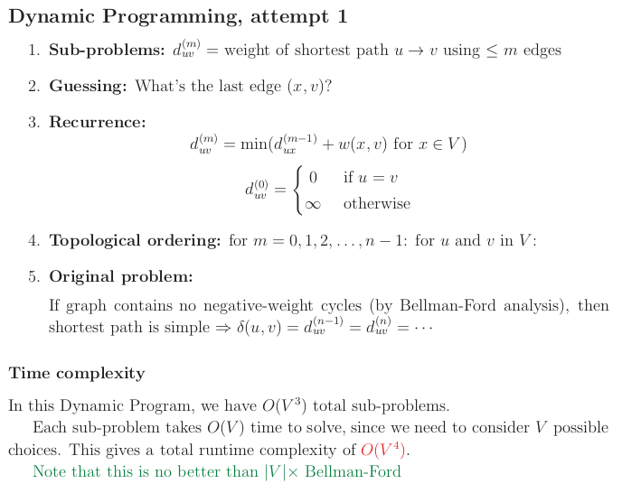
`
CODE
# Bottom-up via relaxation steps
for m = 1 to n by 1
  for u in V
    for v in V
      for x in V # this is the min step
        if duv > dux + dxv # can put wxv too
            duv = dux + dxv
Runtime is , which is the same as running time Bellman Ford.
Matrix Multiplication
Given matrices and compute their product .
- standard algo
- O(n^{2.807}) via Strassen
Matrix multiplication is the same as the above recurrence relation
is similar to for
Define the summation operand to be a min, and the multiplication operand to be .
We can redefine the DP problem using Matrix multiplication language.
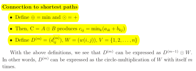
The shortest distance matrix we want to compute equals where the powers is defined in circle land.
All pairs shortest path problem requires computing in circle land. Single matrix multiplication is , hence total complexity is - same algo as above just expressed in another language. However with matrix multiplication you can use repeated squaring trick and get running time .
Floyd-Warshall
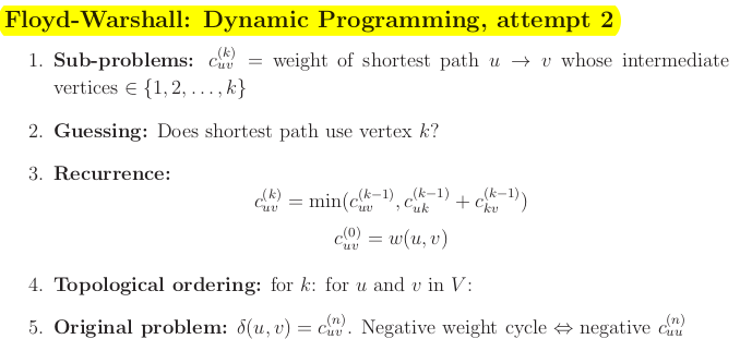
CODE
C = (w(u, v))
for k = 1 to n by 1
  for u in V
    for v in V
      if c uv > c uk + c kv
        c uv = c uk + c kv
Run time
First loop on k, otherwise it will error. k is the phase count.
Jonhson's algorithm
Idea is to do graph re-weighting so that we have nonnegative weights and run Dijkstra. Shortest paths are preserved.
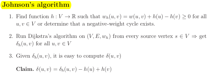
How to find a function ?
You want to find which satisfies for all . This is called a system of difference constraints.
Theorem. If there is a negative-weight cycle, there there exist no solution to the above system.
Theorem. If has no negative-weight cycle, then we can find a solution to the difference constraints.
Proof by example. Add new vertex (source) and connect it to any other vertex and add 0 weights. Compute single source shortest path from and get for every . This is your function . Prooved by triangle inequality.
Time complexity
-
The first step involves running Bellman-Ford from s, which takes time. We also pay a pre-processing cost to re-weight all the edges .
-
We then run Dijkstra’s algorithm from each of the vertices in the graph; the total time complexity of this step is
-
We then need to re-weight the shortest paths for each pair; this takes time.
The total running time of this algorithm is .
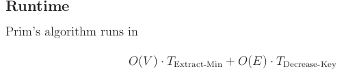
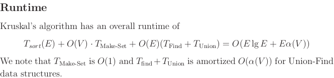
Lecture 12: Greedy Algorithms. Minimum Spanning Tree
- Prim's algorithm
- Kruskal's algorithm
Recall that a greedy algorithm repeatedly makes a locally best choice or decision, but ignores the effects of the future.
Minimum spanning tree problem.
A spanning tree of a graph is a subset of the edges of that form a tree and include all vertices of . Given an undirected graph and edge weights , find a spanning tree of minimum weight sum . We take some edges of the graph, hit all vertices and minimize the weight sum.
Properties of a greedy algorithm:
- Optimal Substructure: the optimal solution to a problem incorporates the optimal solution to subproblem(s)
- Greedy choice property: locally optimal choices lead to a globally optimal solution
In DP you would do guessing, unlike greedy where you are greedy and take the best local option.
Lemma 1. If is a minimum spanning tree of , then is an MST of .
Contract edge - idea. This is to combine two nodes into one and solve the smaller problem.
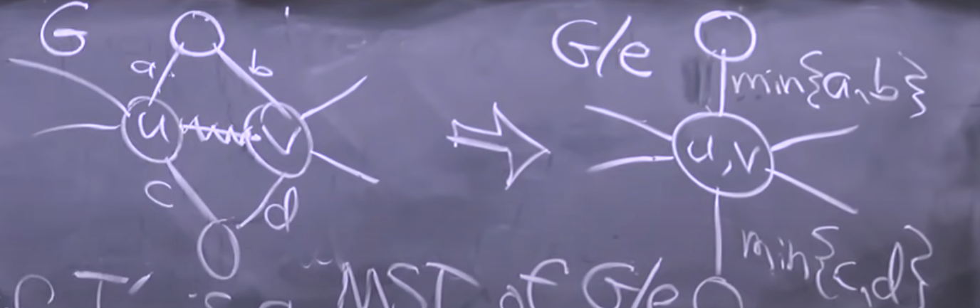
The statement can be used as the basis for a dynamic programming algorithm, in which we guess an edge that belongs to the MST, retract the edge, and recurse. At the end, we decontract the edge and add e to the MST. The lemma proves correctness of the algo but it would be exponential. At each step you guess one random edge of all possible edges.
We need an intelligent way to choose edge .
Lemma 2 (Greedy-Choice Property for MST). For any cut in a graph , any least-weight crossing edge with and is in some MST of .
This lema is your golden ticket to use greedy algo.
Prim's algorithm
It is Dijkstra like.
Idea is to start with one vertex . This is your initial cut vs the rest.
`
CODE
def dist(a,b):
    return abs(a[0]-b[0]) + abs(a[1]-b[1])
h = [(0,0)] # dist,s
edges = {s:float('inf') for s in range(len(points))}
edges[0] = 0
parent = {}
visited = set() # keeps track of your cut, in Dijkstra you do not need that
while h:
    d,s = heappop(h)
    visited.add(s)
    for u in range(len(points)):
        if u not in visited and dist(points[u],points[s]) < edges[u]:
            edges[u] = dist(points[u],points[s])
            parent[u] = s
            heappush(h,(edges[u],u))
# edges has the weights of the MST tree
Runtime just like Dijkstra.
Kruskal's Algoritm
Kruskal constructs an MST by taking the globally lowest-weight edge and contracting it.
sort the edges in nondecreasing weights
for edge in edges:
     add edges consecutively to the DSU in this order (keep tree)
Lecture 13: Incremental Improvement. Max Flow, Min Cut
All about Ford-Fulkerson max-flow algorithm and Max Flow - Min Cut Theorem.
Flow network
Definition. A flow network is a directed graph with two distinguished vertices: a source and a sink . Each edge has a nonnegative capacity . If , then .
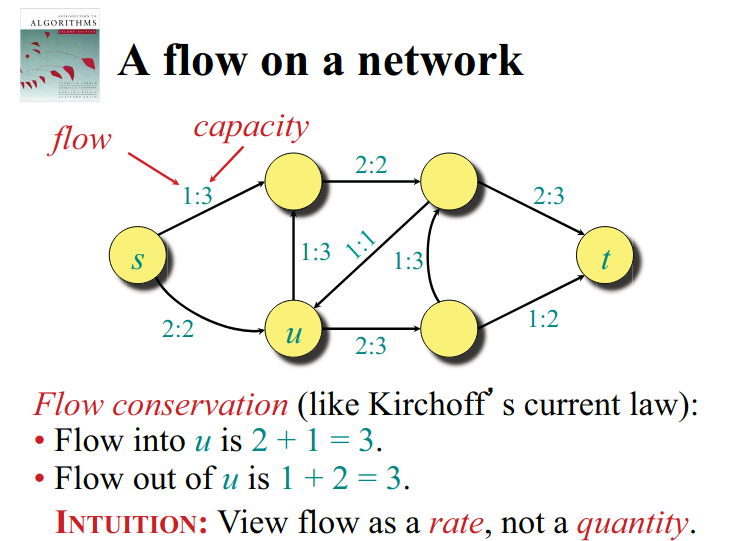
Maximum-flow problem Given a flow network , fund a flow of maximum vale on = max flow rate you can send from source to the sink.
Net Flow
A net flow on is a function satisfying:
- capacity constraint: for all :
- skew symmetry: for all
- flow conservation: for all :
Definition The value of a flow , denoted by is given by
We use implicit summation notation. Example for writing flow conservation:
for all .
Theorem The value of a flow satisfies: , what goes out of the source equals what enters the sink. Proof.
(last step by conservation law)
Cuts
Definition. A cut of a flow network is a partition of such that and . If is a flow on , then the flow across the cut is .
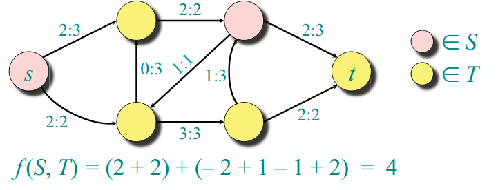
Lemma For any flow and any cut we have Proof
You've got a flow, the flow of the value is the flow value of the cut, as long as you have the source in one place of the cut and the sink on the other part of the cut.
Note because does not contain and we use flow conservation.
Definition The capacity of a cut is
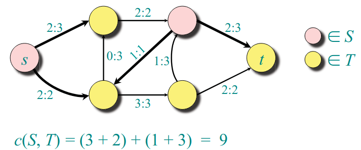
Upper bound on the maximum flow value: Theorem. The value of any flow is bounded above by the capacity of any cut.
Residual network points you where in the network you have free capacities to put flow through. It has the same vertices as the original graph but different edges.
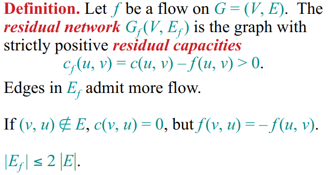
Last two lines above say that your residual network might introduce extra edges which are not in the original network. Residual networks depend on the flow .
Definition Any path from to in is an augmenting path in with respect to . If you have an augmenting path your flow is not a maximum flow. The flow value can be increased along an augmenting path by c_f(p) = min(c_f(u,v)) $ for $(u,v) \in p
Your augmenting path tells you which edges in the original graph with your flow how you change the values on the augmenting path.
Lecture 14: Incremental Improvement. Matching
Max-flow, min-cut theorem
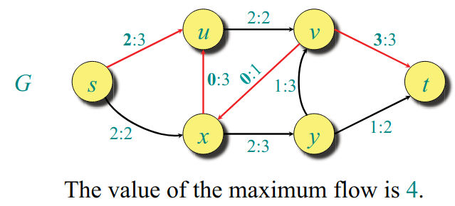
Theorem. The following are equivalent:
- for some cut .
- f is a maximum flow.
- f admits no augmenting paths.
Ford-Fulkerson max-flow algo.
initialize f(u,v) = 9 for all u,v in V
while an augmenting path in G wrt f exists:
  do augment f by c_f(p)
To prove correctness of Ford-Fulkerson we need to prove that 3 implies 2.
We will rove the theorem by proving 3 implies 1, 1 implies 2 and 2 implies 3.
1 implies 2. for any cut. The assumption that shows is a maximum flow as it cannot be increased.
2 implies 3. If there was an augmenting path then the flow value could be increased, hence contradicts that is a maximum flow.
1 implies 3 proof
Ford Fulkerson depends a lot on which augmenting paths you choose every time. Depending on the the order of your Edges, the DFS would choose different augmenting paths. Some of them would have residual flows which are super small and on each augmentation you would add very small flow.
If you do BFS augmenting path search (assuming each edge is of weight 1) then augmentation is proven to be , hence the final run time of the algo is O(VE(V+E))
Baseball elimination
A team survives if it has the largest number of wins. Given a table of standings we want to know which teams still have a chance of surviving.
Check the notes for this example.
Lecture 15: Linear Programming. LP, reductions, Simplex.
You can formulate the max flow problem as an LP problem. LP is more general than Max Flow.
Linear programming (LP) is a method to achieve the optimum outcome under some requirements represented by linear relationships.
LP is polynomial time solvable. Integer LP is NP hard (that is we add extra constraint that the variables are integers).
In general, the standard form of LP consists of
• Variables:
• Objective function:
• Inequalities (constraints): , where is a matrix
and we maximize the objective function subject to the constraints and .
The natural LP formulation of a problem may not result in the standard LP form. Do these transformations:
- Minimize an objective function: Negate the coefficients and maximize.
- Variable xj does not have a non-negativity constraint: Replace with , and , .
- Equality constraints: Split into two different constraints; into .
- Greater than or equal to constraints: Negate the coefficients, and translate to less than or equal to constraint.
Linear Programming Duality
Gives you a certificate of optimality. If I get a solution of the LP problem, I can get a certificate that it is the optimal one (only if indeed it is the optimal one).
For every primal LP problem in the form of:
Maximize c · x
Subject to Ax ≤ b, x ≥ 0,
there exists an equivalent dual LP problem
Minimize b · y
Subject to A^T y ≥ c, y ≥ 0.
The max-flow min-cut theorem can be proven by formulating the max-flow problem as the primal LP problem.
Maximum Flow Given , the capacity for each , the source , and the sink :
Maximize
Subject to skew symmetry
conservation
capacity.
LP could be used for multi-commodity problems.
Shortest Paths
Given , weights for each , and the source , we want to find the shortet paths from s to all , denoted .
Maximize \sum_{v∈V}d(v)

Subject to d(v) − d(u) ≤ w(u,v) ∀u, v ∈ V -  triangular inequality

d(s) = 0.
Note the maximization above, so all distances don’t end up being zero. In the inequalities constrins I have minimim already.
LP Algorithms
- Simplex algorithm
- Ellipsoid algorithm
- Interior Point Method
Simplex The simplex algorithm works well in practice, but runs in ex ponential time in the worst case. Steps:
• Represent LP in “slack” form.
• Convert one slack form into an equivalent slack form, while likely increasing the value of the objective function, and ensuring that the value does not decrease.
• Repeat until the optimal solution becomes apparent.
Slackness is a measure of how tight are our constriants. See Lecture notes for example of algo.
At each step of the simplex algo, you increase the objective value, while maintaining correctness of constraints.
In general, simplex algorithm is guaranteed to converge in choose , iterations where is the number of variables, and is the number of constraints.
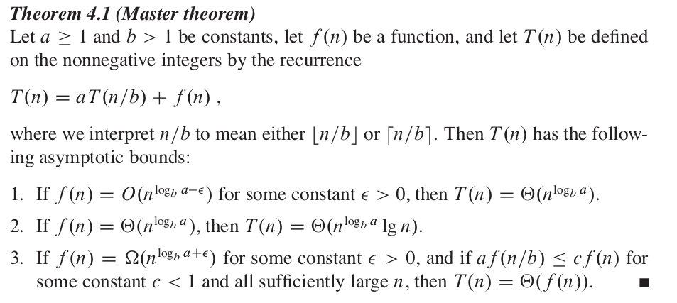
Lecture 16. Complexity: P, NP, NP-completeness, Reductions
P
NP
$NP = $ {decision problems (answer is yes or no) solvable in nondeterministic polynomial time}
Nondeterministic refers to the fact that a solution can be guessed out of polynomially many options in O(1) time. If any guess is a YES instance, then the nondeterministic algorithm will make that guess. NP is biased towards YES.
P vs NP
Does being able to quickly recognize if a solution is correct, means that you can quickly solve the problem?
If yes, then
Sudoku is NP-complete when generalized to a grid.
|Example NP problem. 3SAT
SAT = satisfiability
AT is satisfiability problem - say you have Boolean expression written using only AND, OR, NOT, variables, and parentheses. The SAT problem is: given the expression, is there some assignment of TRUE and FALSE values to the variables that will make the entire expression true?
SAT3 problem is a special case of SAT problem, where Boolean expression should be divided to clauses,such that every clause contains of three literals.
Given a boolean formula of the form where is and and is or. Can you set the variables such that the boolean formula results in True (satisfiable).
This is NP problem beacuse:
- guess x_1 = T or F
- guess x_2 = T or F
If the answer to the SAT3 problem is YES, you can start guessing and then you can check in polynomial time (polynomial verification) if the answer from the guesses is a YES.
NP problems allow you to check the answers in polynomial time.
$NP = $ {decision problems with poly-size certificates and poly-time verifiers for YES outputs}
NP-complete
is NP-complete if \intersect -hard.
is NP-hard if every problem reduces to . X is NP-hard if it is at least as hard as all NP-problems.
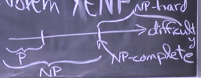
How to prove X is NP-complete.
- Show (come up with polynomial verification)
- Show by reducint from known NP-complete problem from Y to X.
Super Mario Brothers
We show that Super Mario Brothers is NP-hard by giving a reduction from 3SAT.
Dimensional Matching (3DM)
Definition 3. 3DM: Given disjoint sets , and , each of elements and triples is there a subset such that each element is in exactly one triplet ?
3DM is NP. Given a certificate, which lists a candidate list of triples, a verifier can check that each triple belongs to T and every element of X ∪ Y ∪ Z is in one triple.
3DM is also NP-complete, via a reduction from 3SAT.
Subset Sum
Definition 4. Subset Sum Given integers and a target sum , is there a subset such that
Lectures reduce this problem to 3DM and prove it is NP-complete and NP-weakly hard
Partition
Definition 4. Subset Sum Given integers and a target sum , is there a subset such that
reduce it to Subset Sum problem (harday direction) and prove it is NP-complete
Lecture 17. Complexity: Approximation Algorithms
Consider optimization problems. Instead of finding the right answer we approximate the optimal answer.
Definition. An algoithm for a problem of size has an approximation ratio if for any input, the algo produces a solution with cost s.t. where is the cost of the optimal algorithm.
We take the max because the optimization problem can be maximization or minimization.
This says we are a factor of from an optimal solutions.
Definition. An approximation scheme that takes as input $eps > 0$ and produces a solution such that for any fixed , is a -approximation algorithm.
if PTAS is polynomial time approximation scheme.
O(n/\eps}) if FPTAS is fuly polynomial time approximation scheme.
Vertex Cover
For an undirected graph find a smallest subset of vertices such that all edges are covered. An edge is covered if one of its endpoints is in the subset of vertices. (NP-complete)
Heuristics:
- pick maximum degree vertex
- pick random edge , then remove all incident edges to
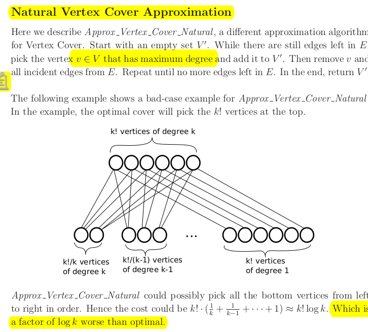
- pick random edge , then remove all incident edges to is a factor of 2 apart from the optimal solution. All edges we pick are disjoint and if the number of edges we pick in the end is A, then the number of vertices is 2A.
Set Cover
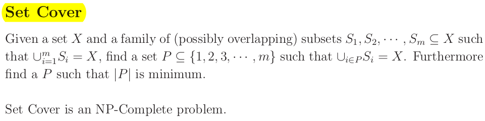
Heuristic: pick subset which covers the most uncovered elements.
Algo:
Start by initializing the set to the empty set. While there are still elements in X,4 pick the largest set $S_i and add to . Then remove all elements in from and all other subsets . Repeat until there are no more elements in .
Claim: This is a -approximation algorithm (where ).
Partition
Given a set of elements, split it into two subsets and minimize the max of the sums of the two subsets. This is an NP-Complete problem.
Partition problem
Multiway partition problem
Approximation algo.
Phase 1. For smaller subset of size find optimal solution using brute force . You get two subsets and .
Phase 2. For the rest of the elements add greedily one by one.
If m = ) then this is -approximation algo.
Lecture 18. Complexity: Fixed-Parameter Algorithms
Last 3 lectures:
Pick any two:
- solve hard problems
- solve them fast (poly-time)
- exact solution
Idea: Aim for exact algorithm, but confine exponential depedence to a parameter.
Parameter: A parameter is a nonnegative integer k(x) where x is the problem input. The parameter is a measure of how tough is the problem you are solving.
Parameterized Problem: A parameterized problem is simply the problem plus the parameter or the problem as seen with respect to the parameter.
Goal: Algo is polynomial in problem size , exponential in parameter .
Vertex Cover Problem Given a graph and non-negative integer . Question: is there a vertex cover of size not greater than
This is a decision problem for Vertex Cover and is also NP-hard.
Obvious choice of parameter is . (natural parameter)
Brute force
Try all choose subsets of vertices., test each for coverage. Running time is
exponent depends on this is slow. I cannot say that for any fixed the algo is quadratic for example.
Fixed Parameter Tractability
A parameterized problem is fixed-parameter tractable (FPT) if there is an algorithm with running time , such that (non negative) and is the parameter, and the degree of the polynomial is independent of and .
Question: Why and not ? Theorem: algorithm iff
vertex cover problem is FPT:
- pick random edge
- either or or both is in the subset
- guess each one:
- add to , delete u an all incident edges from G, recurse with
- do the same but with instead of
- return the of the two outcomes
Recursion tree:
                (n,k)
      (n-1,k-1)       (n-1,k-1)
(n-2,k-2) (n-2,k-2) (n-2,k-2) (n-2,k-2)
base case when return true if no edges, else false. At each node we do work to delete incident edges. The total runtime is
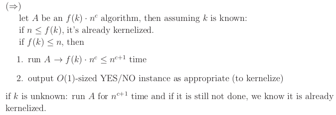
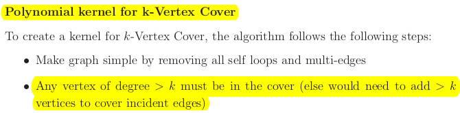
Kernalization is a polynomial time algorithm that converts an input into a small and equivalent input . Equivalent means that the answer I get in the end are the same. We want . The algo you run on the smaller input would not depend on anymore, your problem size depends on , hence your running time is O(kernalization) + O(run on smaller input) = .
Theorem Aproblem is FPT iff there exists a kernelization.
Kernelize -> FPT is trivial.
Lecture 19. Synchronous Distributed Algorithms: Symmetry-Breaking. Shortest-Paths Spanning Trees
What are Distributed Algorithms?
Algorithms that run on networked processors, or on multiprocessors that share memory.
Most computing is on distributed systems.
Difficulties:
- concurrent activities
- uncertainty of timing
You have a different way of framework for thinking about problems here. You cannot just solve graph problems the usaul way you do, e.g. storing everything in adjacency list or matrix. All nodes are similar and you are allowed to send messages. By sending messages across the network you solve algos.
We consider two distributed computing models: • Synchronous distributed algorithms:
- Leader Election
- Maximal Independent Set
- Breadth-First Spanning Trees
- Shortest Paths Trees • Asynchronous distributed algorithms:
- Breadth-First Spanning Trees
- Shortest Paths Trees
Distributed Network
Based on an undirected graph associate:
- a process with each graph vertex
- two directed communication channels with each edge
Processes at nodes communicating using messages.
Each process has output ports, input ports that connect to communication channels.
Select a leader node in a distributed system.
Theorem 2: Let be an -vertex clique. Then there is an algorithm consisting of deterministic processes with UIDs that is guaranteed to elect a leader in . The algorithm takes only 1 round and uses only point-to-point messages.
• Algorithm:
- Everyone sends its UID on all its output ports, and collects UIDs received on all its input ports.
- The process with the maximum UID elects itself the leader.
Maximal Independent Set
Problem: Select a subset of the nodes, so that they form a Maximal Independent Set.
- Independent: No two neighbors are both in the set.
- Maximal: We can’t add any more nodes without violating independence.
Need not be globally maximum, you just need to have local independence. Can have more than one MIS sets.
Distributed MIS?
You have a graph representing the distributed system. The problem of finding an MIS in distributed system is not the same as gather all nodes and edges and run algo. Here each node should know if it is in the MIS or not using messages.
Assume:
- No UIDs
- Processes know a good upper bound on .
Require:
- Compute an MIS of the entire network graph.
- Each process in should output in, others output out.
Luby’s MIS Algorithm
• Executes in 2-round phases.
• Initially all nodes are active.
• At each phase, some active nodes decide to be in, others decide to be out, algorithm continues to the next phase with a smaller graph.
• Repeat until all nodes have decided.
• Behavior of active node at phase :
• Round 1:
- Choose a random value in , send it to all neighbors.
- Receive values from all active neighbors.
- If is strictly greater than all received values, then join the MIS, output in.
• Round 2: – If you joined the MIS, announce it in messages to all (active) neighbors. – If you receive such an announcement, decide not to join the MIS, output out. – If you decided one way or the other at this phase, become inactive.
Termination
• With probability 1, Luby’s MIS algorithm eventually terminates.
• Theorem 7: With probability at least , all nodes decide within phases.
• Proof uses a lemma similar to before: • Lemma 8: With probability at least , in each phase 1, ... , , all nodes choose different random values.
• So we can essentially pretend that, in each phase, all the random numbers chosen are differet.
• Key idea: Show the graph gets sufficiently “smaller” in each phase.
• Lemma 9: For each phase ph, the expected number of edges that are live (connect two active nodes) at the end of the phase is at most half the number that were live at the beginning of the phase.
Formal proof with probability bounds and expectation in slides. Animation of Luby algo in slides.
Breath-First Spanning Trees
That's the tree you get from BFS.
• New problem, new setting.
• Assume graph G = (V, E) is connected.
• V includes a distinguished vertex , which will be theorigin (root) of the BFS tree.
• Generally, processes have no knowledge about the graph.
• Processes have UIDs.
- Each process knows its own UID.
- is the UID of the root .
- Process with UID io knows it is located at the root.
• We may assume (WLOG) that processes know the UIDs of their neighbors, and know which input and output ports are connected to each neighbor.
• Algorithms will be deterministic (or nondeterministic), but not randomized.
Output: Each process should output parent , meaning that ’s vertex is the parent of ’s vertex in the BFS tree.
Very similar strategy to standard BFS just need to add te sending and hearing messages part.
Termination
• Q: How can processes learn when the BFS tree is completed?
• If they knew an upper bound on diam, then they could simply wait until that number of rounds have passed.
• Q: What if they don’t know anything about the graph?
When a subtree finishes propagate upwards that you are done, this starts from the leaves and goes upward. Need to send information up on the tree.
Need to send info upwards the tree.
Lecture 20. Asynchronous Distributed Algorithms: Shortest-Paths Spanning Trees
Synchronous Network Model
- Processes at graph vertices, communicate using messages.
- Each process has output ports, input ports that connect to communication channels.
- Algorithm executes in synchronous rounds.
- In each round:
- Each process sends messages on its ports.
- Each message gets put into the channel, delivered to the process at the other end.
- Each process computes a new state based on the arriving messages.
The way of thinking in distributed systems is fundamentally different. You have a string limitation that every node in the system knows only things about itself and its neighbourhood. It is not aware of the whole system.
Each node of the graph has some process which is not aware of how the graph looks like. Nodes are connected through channels
Asynchronous Network Model
-
Complications so far:
- Processes act concurrently.
- A little nondeterminism.
-
Now things get much worse:
- No rounds---process steps and message deliveries happen at arbitrary times, in arbitrary orders.
- Processes get out of synch.
- Much more nondeterminism.
Asynchronous networks complexity:
-
Message complexity is number of messages sent by all processes during the entire execution
-
Time complexity. Cannot measure rounds like in synchronous networks.
-
A common approach:
-
Assume real-time upper bounds on the time to perform basic steps:
- for a channel to deliver the next message, and
- for a process to perform its next step. (local processing time)
Infer a real-time upper bound for solving the overall problem.
Now we have a big machine (queue) where each process is somewhere in the queue. As they execute we push and dequeu from the queue of processes.
BFS in asynchronous model
If you run simply the BFS like in synchronous model you might end up with a tre which is not BFS-output tree and do not have the shortest paths:
Message complexity:
Number of messages sent by all processes during the entire execution.
Time complexity:
Time until all processes have chosen their parents. Neglect local processing time.
- Q: Why diam, when some of the paths are longer? To have long paths these processes must run faster than the diameter path.
To fix it you need a relaxation algorithm, like synchronous Bellman-Ford.
Strategy:
- Each process keeps track of the hop distance, changes its parent when it learns of a shorter path, and propagates the improved distances.
- Eventually stabilizes to a breadth-first spanning tree.
Shortest Paths
- Use a relaxation algorithm, once again. (same as synchronous but would be slower)
- Asynchronous Bellman-Ford.
- Now, it handles two kinds of corrections:
- Because of long, small-weight paths (as in synchronous Bellman-Ford).
- Because of asynchrony (as in asynchronous Breadth-First search).
• The combination leads to surprisingly high message and time complexity, much worse than either type of correction alone (exponential).
Lecture 21. Cryptography: Hash Functions
A hash function maps arbitrary strings of data to fixed length output. We want it to look random. In practice, hash functions are used for “digesting” large data.
, the stars says that we can have arbitrary long string of bits.
No secret keys, all is public. Anyone can compute .
Goal: Make run fast (polytime) and make it hard to have collisions. Simple stuff with mod is but is easy to find colissions.
We want to approximate/create a random oracle with these properties:
- For input , if has not seen before, then it outputs a random value , Else returns its previously output.
- the random oracle gives a random value (get it by throw a coin 256 times (SHA-256)), and gives deterministic answers to all inputs it has seen before.
Desirable Properties
- One-way (pre-image resistance): Given , it is hard to find an x such that .
- Strong collision-resistance: It is hard to find any pair of inputs such that .
- Weak collision-resistance (target collision resistance, 2nd pre-image resistance): Given , it is hard to find such that .
- Pseudo-random: The function behaves indistinguishable from a random oracle.
- Non-malleability: Given , it is hard to generate (without using )for any function .
Lecture 22. Cryptography: Encryption
Symmetric key encryption
- secret key assume is 128 bit. It is shared between Alice and Bob.
stands for ciphertext, is message (plaintext), is the encryption function, is descryption function.
and need to be reversible operations (plus, minus, permutation, shift left, right)
Key exchange
How does secret key get exchanged/shared?
Puzzle: Alice sends to Bob a box with money, but need to be locked otherwise it would get stolen.
Solution: A locks the box sends to Bob. Bob locks the box and sends to Alice. Alice unlocks her lock and sends back to Bob.
Math assumption: Communitivy tbetween the lockers. Locking a box within a Box would not work.
Diffie-Hellman Key Exchange
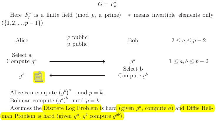
is Alice's locker that hides , is Bob's locker that hides . The goal is Alice and Bob share secretly the key . Middle man Mal might put their own locker , thus we need asymmetric encryptions, Alice needs a way to authenticate she is communicationg with Bob. Authenticate using public/private key enctyption
Public Key encryption
Bob comes up with public and private keys. Alice sends to Bob cipher text.
message + public key = ciphertext ciphertext + private key = message
The two keys need to be linked in a mathematical way. Knowing the public key should tell you nothing about the private key.
RSA encryption algorithm.
- Alice picks two large secret primes and
- Alice computes
- Alice chooses an encryption exponent s.t.
- Alice public key is a tuple
- Dectyption exponent obtained using Extended Euclidean Algorithm by Alice (secretly) such that
- Alice private key
Encryption and Decrypton with RSA
- encryption
- descryption
To prove it works we need to show that
Hardness of RSA
• Factoring: given , hard to factor into .
• RSA Problem: given such that gcd and , find such that mod . Breaking a particular encryption .
The factoring problem: Given find and , is unknown if is -complete. Weird.
Other problems and knapsack are NP-complete and have been used in crypto algos but have been all broken and do not work in practice.
This is because NP-completeness is telling you stuff about the worse case. For cryptography we want probblems to have hard problems on average.
Lecture 23. Cache-Oblivious Algorithms: Medians & Matrices
In all algos so far we assumed accessing different data cost the same.
Modern Memory Hierarchy
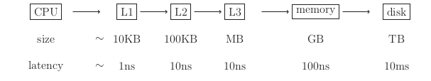
The closer to the CPU the faster you can transfer data.
Two notion of speed:
- latency (how quickly you can fetch data)
- bandwidth (how fat are the pipes between different hierarchies)
longer latency due to lnger distance data need to travel
A common technique to mitigate latency is blocking: when fetching a word of data, get the entire block containing it.
Amortize latency over a whole block.
Cost for getting one data point over a block:
latency/block size + 1/bandwidth
Block should have useful elements. We require the algorithm to use all words in a block (spatial locality) and reuse blocks in cache (temporal locality).
Exteranal Memory Model
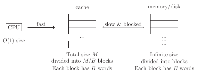
Assume:
- cache access is free
- disk is huge (infinitely large)
This model handles blocks explicitly.
We count number of memory transfers between cache and the disk.
Cache-oblivious Model
The only change from the external memory model is that the algorithm no longer knows and . Accessing a word in the memory automatically fetches an entire block into the cache, and evicts the least recently used (LRU) block from the cache if the cache is full.
Different computers might have different and .
External and Cache-oblivious models give you a way to measure the data transfer complexity of algorithms.
Scanning
for i in range(N):
  sum += A[i]
Assume is stored contiguously in memory. Arrays are stored in contiguous parts of the memory, dictionaries not. This is why DICTIONARIES READ AND WRITE is much SLOWER
External memory model can align with a block boundary, so it needs memory transfers.
Cache -oblivious algorithms cannot control alignment (because it does not know B), so in needs memory transfers. cound be 2 and these two elements could be at a boundary, so you would need to access 2 blocks of memory.
Divide and Conquer
Base case:
- problem fits in cache
- problem fits in blocks,
Median Finding
- view array as partitioned into columns of 5 (each column is size).
- sort each column
- recursively find the median of the column medians
- partition array by x
- recurse on one side
We will now analyze the number of memory transfers in each step. Let be the total number of memory transfers.
- free
- a scan,
- , this involves a pre-processing step that coallesces the elements in a consecutive array
- 3 parallel scans, , read all elements, check those less than , check those greater than
Lecture 24. Cache-Oblivious Algorithms: Searching & Sorting
Why LRU block replacement strategy?
is the size of the Cache size
is the number of block evictions(i.e. number of block reads)
OPT knows the future and gives the most optimal eviction policy which minimizes the number of evictions.
Proof in lecture notes.
Final notes on other classes.
- 6.047 - Computational Biology
- 6.854 - Advanced Algorithms (natural class to take after this one)
- 6.850 - Computational Geometry
- 6.849 - Folding algorithms
- 6.851 - Advanced Datastructure
- 6.852 - Distributed Algorithms
- 6.853 - Algorithms on game theory
- 6.855 - Network optimization
- 6.856 - Randomized algorithms
- 6.857 - Applied cryptography
- 6.875 - Theoretical cryptography
- 6.816 - Multicore programming
- 6.045 - Theory of computation classes (NP complete stuff, complexity)
- 6.840 - Theory of computation grad class
- 6.841 - Advanced complexity theory
- 6.842 - Randomized complexity theory
- 6.845 - Quantom complexity thery
- 6.440 - Coding theory