Neural Networks and Deep Learning

Coursera course by Andrew Ng

This is a course part of the Deep Learning Specialization

Intro to DL

ReLU = Rectified Linear Unit: $max(0,wx+b)$

Hidden Layers of a neural network learn more complex patterns in your data. The magic of NN is that you do not need to learn explicitly what are these patters.

Every hidden layer is a complex function of the input layer.

Applications of different DL

• Standard NN, Feed Forward NN: Home prices, Ad prediction
• CNN: images
• RNN: sequential data (audie, NLP, language, translation), temporal component

Structured data = tabular

Unstructured data = text, images, audio,

Why DL is taking off now?

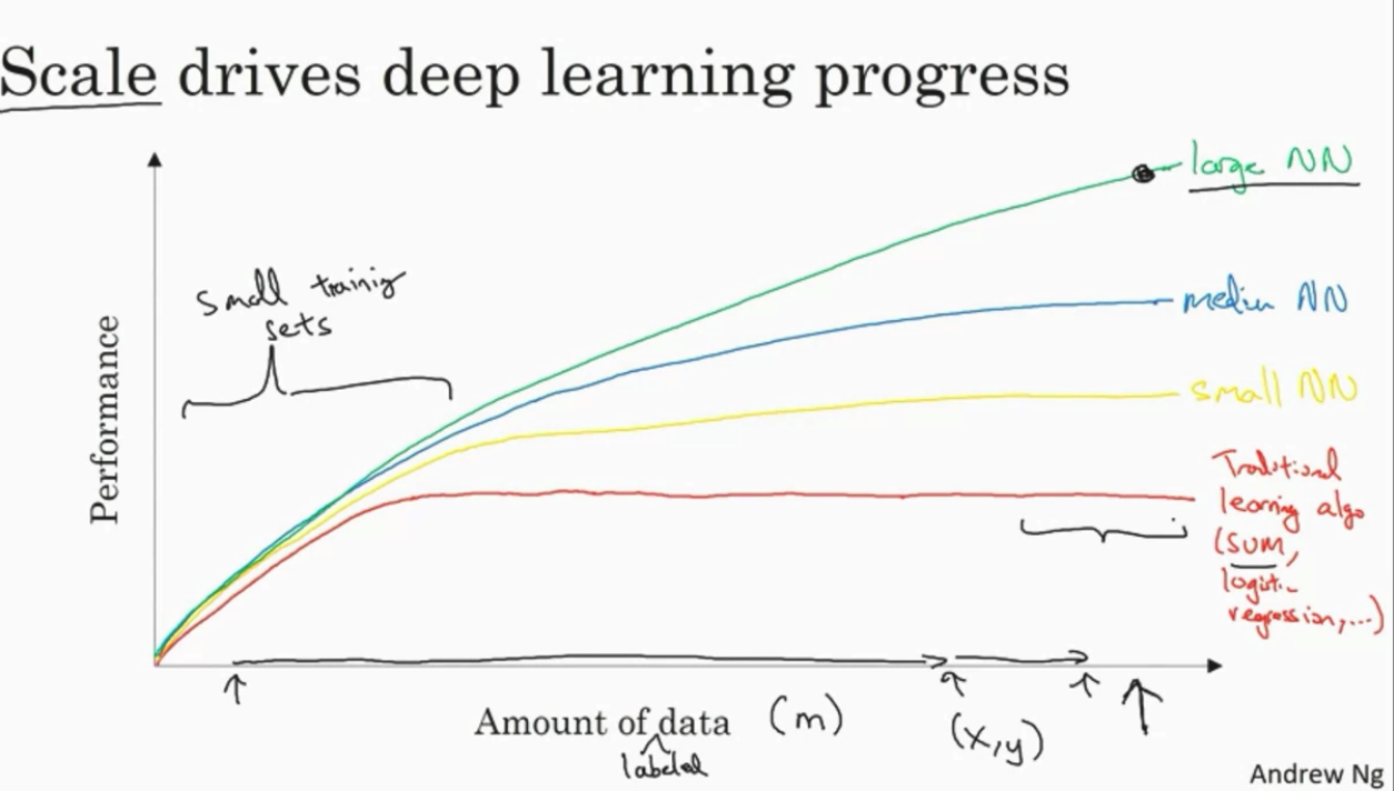
When data is small, the rank of ML/DL algos depends much on your skills on modelling and architecture building. When data is big, usually NN are better.

Innocations:

• More data
• faster computation (CPU, GPU...)
• better algorithms

Sigmoid activation function to RELU the computation is much faster, Relu has gradient 1 for positive values, sigmoid can have gradient close to 0.

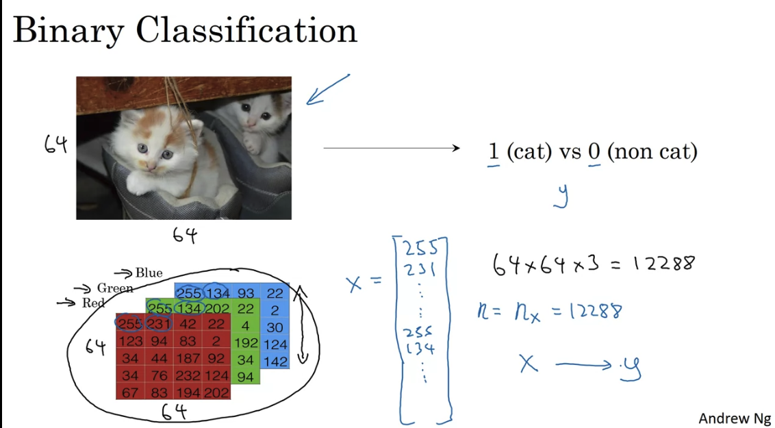
Logistic Regression as a Neural Network

Binary classification of an image - flatten all pixels into one vector

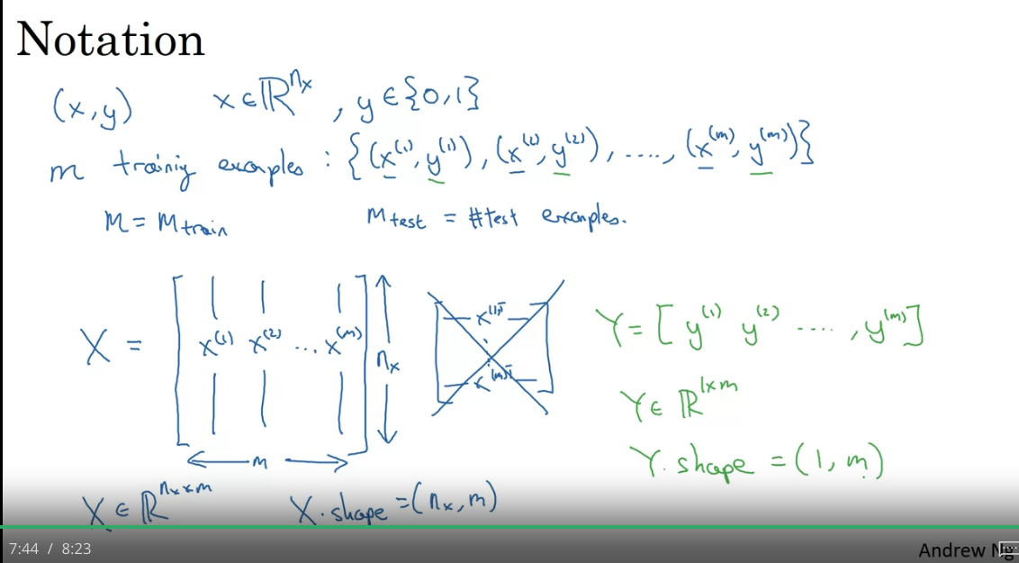
In NN the design matrix would have dimension $nxm$ - it is easier that way (transposed of ML design matrix)

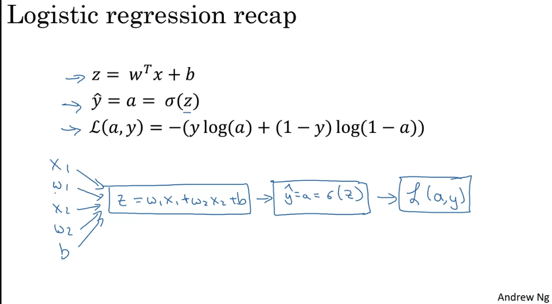
Logistic regression is just applying sigmoid function to the linear model, $\hat{y} = \sigma(wx+b)$ and using logistic loss function.

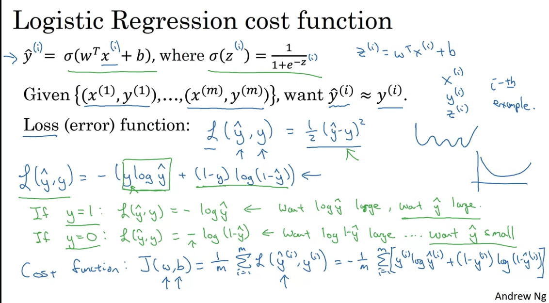
Note in logistic regression we predict $\hat{y} = \sigma(wx+b)$ which represents a probability between 0 and 1. We use the ogistic losss function so that we have a convex cost function. No matter where you initialize, you would reach the global minimum.

Logistic loss = - Log likelihood

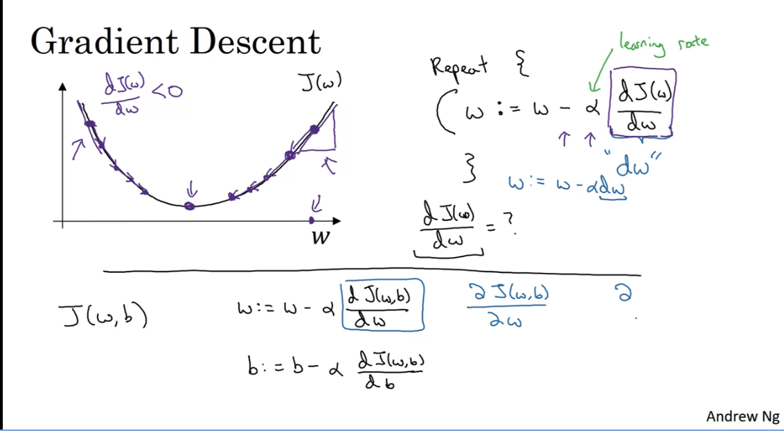
Gradient Descent

$w = w-\alpha J'(w)$, where J is the loss function

The gradient is equal to the slope of the tangent function. Math derivation:

Say for $f(x)$ you want to find the tangent line $ax+b$ at point $x_1$

Then $f(x_1) = ax_1+b$ must have one solution. Take derivative of both sides:

$a=f'(x_1)$

Note that at each step we go to the opposite direction of the derivative with a step size of $\alpha$. By the graph above you can see how we slowly go to the optimum value. You can use also only the sign of the derivative. But using the derivative itslef gives you smaller stepsize when you are closer to the optimum value.

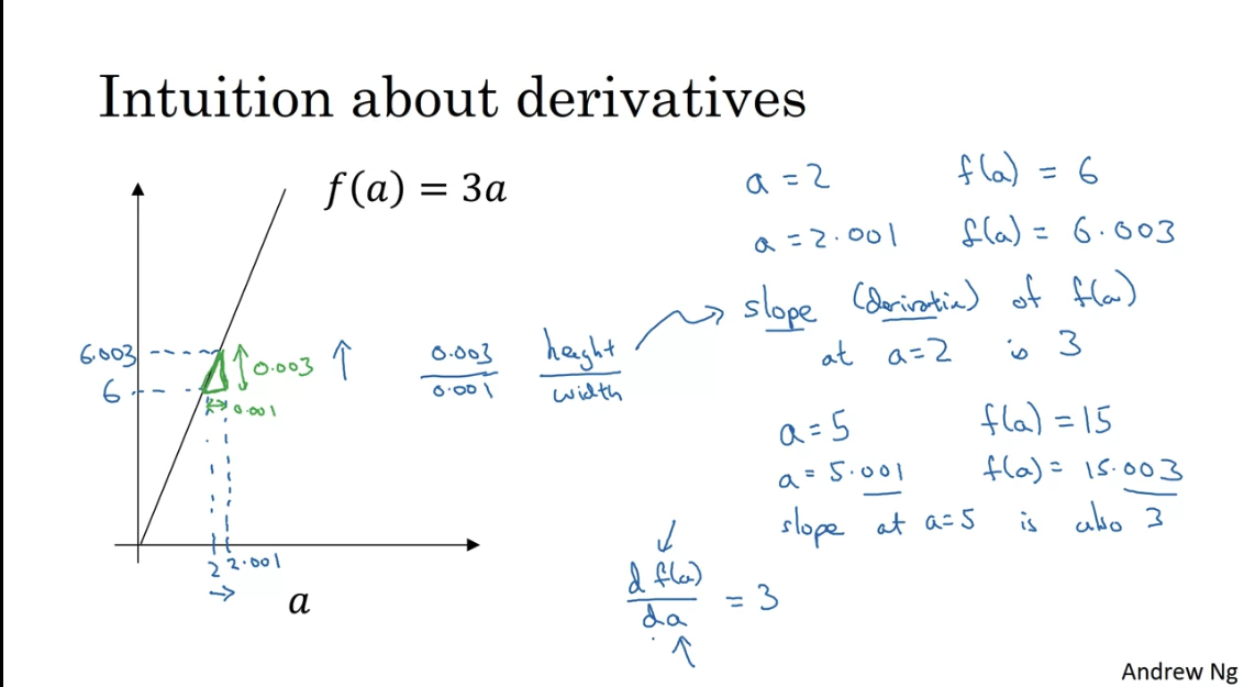
Derivative = slope = change in $f$/ change in $x$ = how much $f$ would change if you change $x$ by a little bit. In the picure above if you nudge $a$ by 0.001, then $f$ changes by 0.003

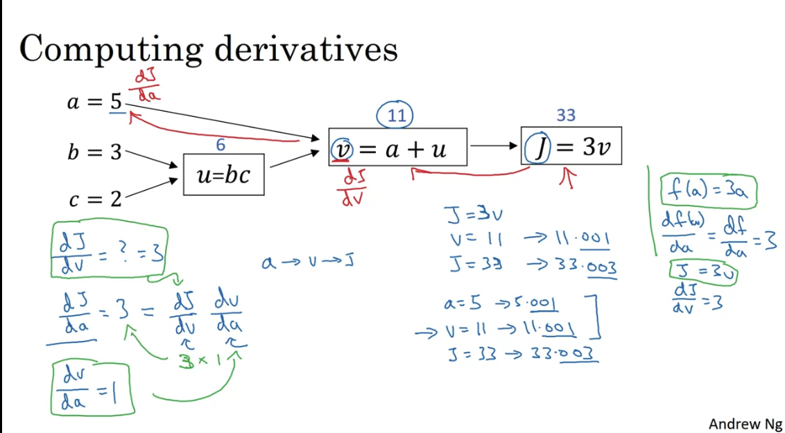
Computation Graph

NN are organised in terms of:

• forward propagation: compute output of NN
• backward propagation: compute gradient of the loss function with respect to parameters

The computation graph organises these two steps.

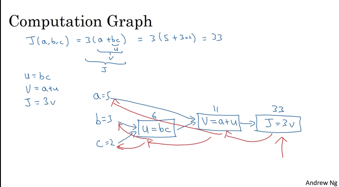
Backprogation is just an application of the chain rule.

Changing $v$ by 0.001, $J$ changes by 0.003, hence $dJ/dv = 3$. When you change $a$ by 0.001, $J$ changes by 0.003, hence $dJ/da = 3$. But also changing $a$ changes $v$ which changes $J$. $dJ/da = dJ/dv dv/da$. This is the chain rule.

Logistic regression computational graph

$a=\hat{y}$ below

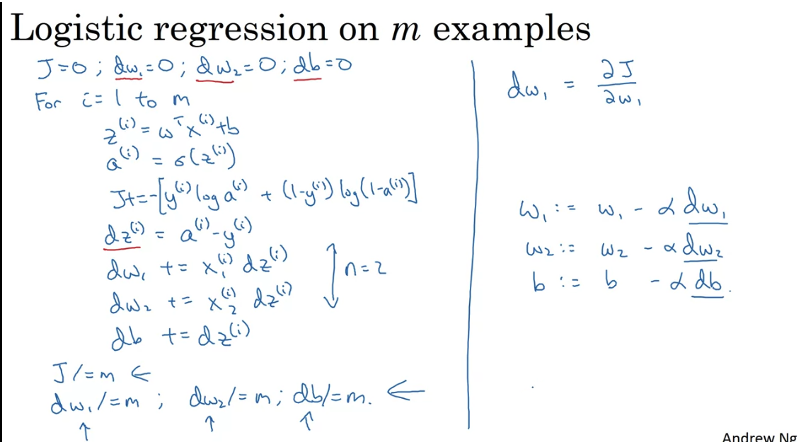
Goal is to compute $dJ/dw$, $dJ/db$, $dJ/dz$, $dJ/da$, where the first two are the gradients of the loss function with respect to the parameters, and the last two are the gradients of the loss function with respect to the intermediate variables.

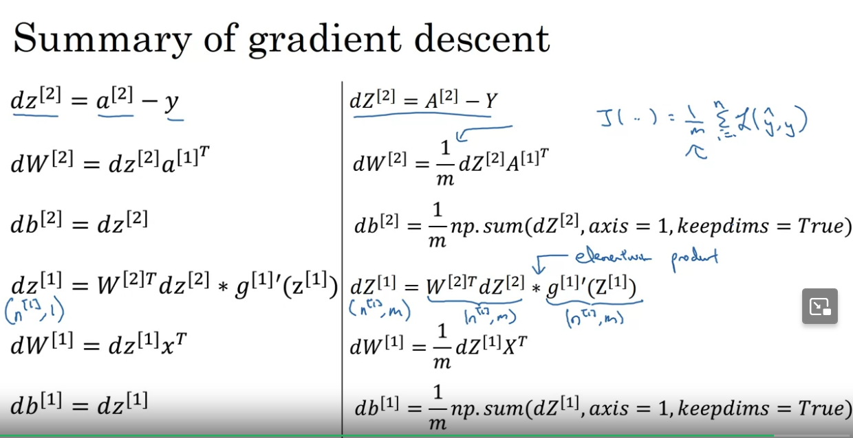
One step gradient descent for logistic regression gradient descent:

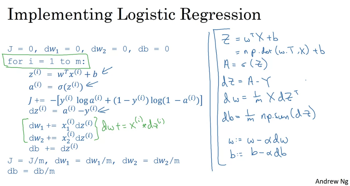
Vectorization

Great speedups. Instead of looping over all examples, you can do the computation in one go.

Broadcasting in Python

Broadcasting copies automatically the vector to the right shape. For example:

np.array([1,2,3,4]) + 100 = np.array([101,102,103,104])
np.array([1,2,3,4],[5,6,7,8]) + 100 = np.array([101,102,103,104],[105,106,107,108])

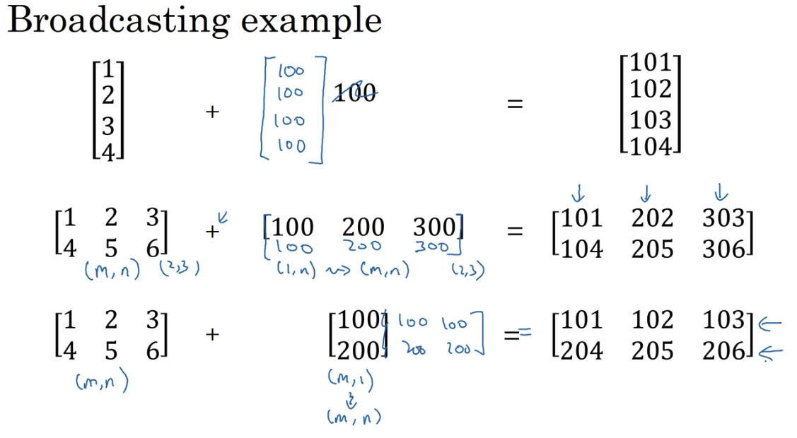
$3x4$ matrix division by $1x4$ vector gives $3x4$ matrx

NOTE on vectors Use:

np.random.rand(5,1) # shape is (5,1) - column vector

Do not use:

np.random.rand(5) # shape is (5,) - that is nothing

Tip:

• add assert statements to check the shape of the vectors

asser (w.shape == (n,1))

Remember:

• the sigmoid function and its gradient $\sigma'(x)=\sigma(x)*(1-\sigma(x))$
• image2vector is commonly used in deep learning
• np.reshape is widely used. In the future, you'll see that keeping your matrix/vector dimensions straight will go toward eliminating a lot of bugs.
• numpy has efficient built-in functions
• broadcasting is extremely useful

Shallow Neural Networks

For one training sample:

One hidden-layer NN = Two layer NN (inpuut layer is not ussually counted)

First layer: $z^{[1]} = Wx + b$, $a^{[1]} = \sigma(z^{[1]})$

Second layer: $z^{[2]} = Wa^{[1]} + b$, $a^{[2]} = \sigma(z^{[2]})$

Assume we have $n_x$ input features, $n_h$ hidden units, $n_y$ output units. Then the dimensions of the matrices are: $W^{[1]}$ is $n_h$ x $n_x$, $b^{[1]}$ is $n_h$ x $1$, $W^{[2]}$ is $n_y$ x $n_h$, $b^{[2]}$ is $n_y x 1$.

For multiple training sample:

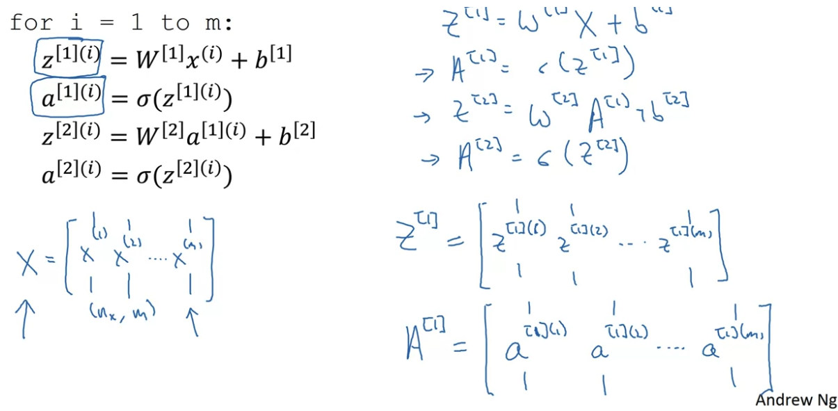
This shows why we have the design matrix X dimensions to be dimension x training_samples (mxn)

Activation functions

• sigmoid: $\sigma(z) = \frac{1}{1+e^{-z}}$ goes between 0 and 1
• tanh: $\tanh(z) = \frac{e^z-e^{-z}}{e^z+e^{-z}}$ goes between -1 and 1
• ReLU: $a = max(0,z)$
• leaky ReLU = $max(0.01z,z)$ tanh would make your hidden layers have mean around 0.

Andrew Ng: "tanhh is almost always better than sigmoid function, except for the output layer where you have to predict 0 or 1. In that case, sigmoid is better. I almost never use sigmoid function as activation function in hidden layers."

Downside of both sigmoid and tanh is that if $z$ is large than the derivative/slope is almost equal to 0 (vanishing gradient).

ReLU has derivate 1 when z is positive and 0 when it is negative. If $z=0$ then the derivative is not defined (which does not happen in practice)

Rule of thumb: "ReLU is the default activation function to use if you don't know what activation function to use for hidden layers. For output layer, sigmoid for binary classification, sigmoid for multi-class classification, and no activation for regression."

Leaky ReLU is used when you have a lot of negative values in $z$ and you want to avoid the "dead neurons" problem. But in practice ReLU is used more often.

ReLU is used more often than tanh because the slope is very different than 0 for positive values of $z$ and NN learns much faster.

Sigmoid is almost never used for hidden layers

ReLU is the most common activation function

You need linear activation function for the output layer for regression problems. Otherwise, on hidden layers there is no point using linear activation function because the NN would be just a linear function (compozition of linear functions is linear).

Derivatives of activation functions

• sigmoid: $\sigma'(z) = \sigma(z)*(1-\sigma(z))$, derivative at 0 is $1/4$
• tanh: $\tanh'(z) = 1 - \tanh^2(z)$, $z = 0$, then $tanh'(z) = 1$

Gradient descent in NN with 1 hidden layer

NN require random initialization of the weights. If they are all 0-s then all activation functions in one layer would be the same values.

Initialization when using sigmoid on tanh it might be better to initailize wth random values which are smaller (for large z the derivative vanishes)

Reminder: The general methodology to build a Neural Network is to:

1. Define the neural network structure ( # of input units, # of hidden units, etc).
2. Initialize the model's parameters
3. Loop:
   • Implement forward propagation
   • Compute loss
   • Implement backward propagation to get the gradients
   • Update parameters (gradient descent)

Deep Neural Networks

The deeper the layr the more complex features can be learned. For example in images:

• input layer - pixels
• first layer learns edges
• second layer learns shapes
• third layer learns parts of objects
• fourth layer learns objects
• fifth layer learns scenes
• output

Theory

There are functions which can be represented by a deep NN with a small number of hidden units, but require an exponential number of hidden units in a shallow NN.

Layer $l$: $W^{[l]}$ weights, $b^{[l]}$ bias

Input: $a^{[l-1]}$, output: $a^{[l]}$

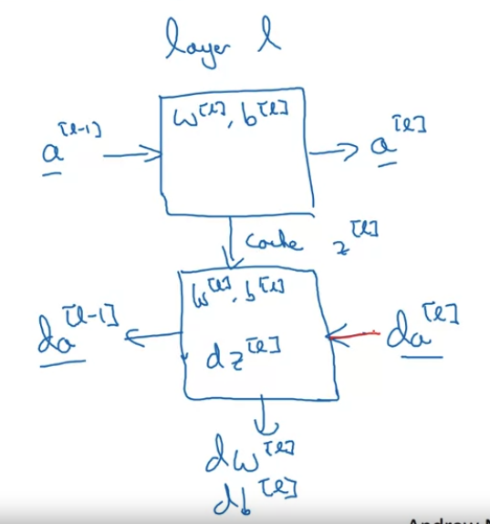
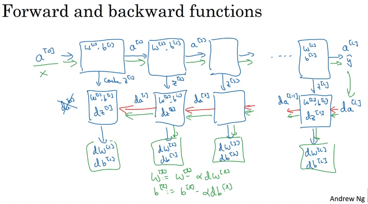
Forward and backward propagation

Deep Learning is good at learning very flexible and complex functions.

DL and NN has nothing to do with the brain. It is just a function approximation algorithm. Neuro science is not very useful for DL - we do not even know how neurons work in the brain.

Implementation of DL

Steps:

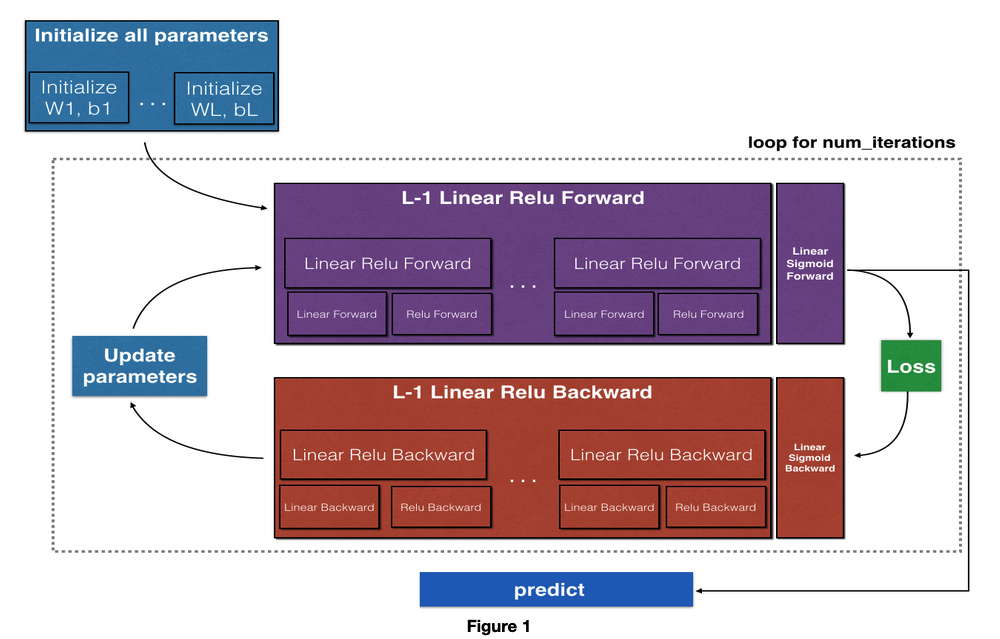
• Initialize the parameters for a two-layer network and for an $L$-layer neural network
• Implement the forward propagation module (shown in purple in the figure below)
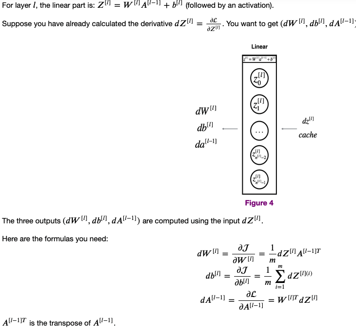
  • Complete the LINEAR part of a layer's forward propagation step (resulting in $Z^{[l]}$).
  • The ACTIVATION function is provided for you (relu/sigmoid)
  • Combine the previous two steps into a new [LINEAR->ACTIVATION] forward function.
  • Stack the [LINEAR->RELU] forward function L-1 time (for layers 1 through L-1) and add a [LINEAR->SIGMOID] at the end (for the final layer $L$). This gives you a new L_model_forward function.
• Compute the loss
• Implement the backward propagation module (denoted in red in the figure below)
  • Complete the LINEAR part of a layer's backward propagation step
  • The gradient of the ACTIVATION function is provided for you(relu_backward/sigmoid_backward)
  • Combine the previous two steps into a new [LINEAR->ACTIVATION] backward function
  • Stack [LINEAR->RELU] backward L-1 times and add [LINEAR->SIGMOID] backward in a new L_model_backward function
• Finally, update the parameters

Note:

For every forward function, there is a corresponding backward function. This is why at every step of your forward module you will be storing some values in a cache. These cached values are useful for computing gradients.

In the backpropagation module, you can then use the cache to calculate the gradients.

def initialize_parameters(n_x, n_h, n_y):
    """
    Argument:
    n_x -- size of the input layer
    n_h -- size of the hidden layer
    n_y -- size of the output layer
    
    Returns:
    parameters -- python dictionary containing your parameters:
                    W1 -- weight matrix of shape (n_h, n_x)
                    b1 -- bias vector of shape (n_h, 1)
                    W2 -- weight matrix of shape (n_y, n_h)
                    b2 -- bias vector of shape (n_y, 1)
    """
    
    np.random.seed(1)
    
    #(≈ 4 lines of code)
    W1 = np.random.randn(n_h, n_x)*0.01
    b1 = np.zeros((n_h, 1))
    W2 = np.random.randn(n_y, n_h)*0.01
    b2 = np.zeros((n_y, 1))
    # YOUR CODE STARTS HERE
    
    
    # YOUR CODE ENDS HERE
    
    parameters = {"W1": W1,
                  "b1": b1,
                  "W2": W2,
                  "b2": b2}
    
    return parameters  

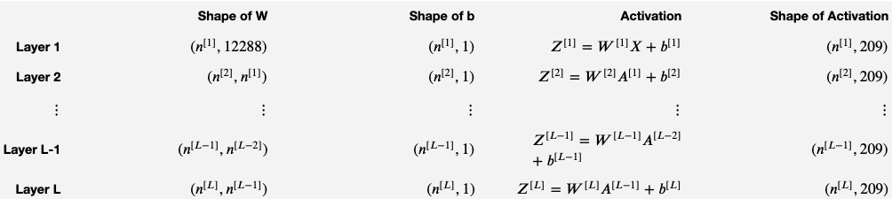
The initialization for a deeper L-layer neural network is more complicated because there are many more weight matrices and bias vectors. When completing the initialize_parameters_deep function, you should make sure that your dimensions match between each layer. Recall that $n^{[l]}$ is the number of units in layer $l$. For example, if the size of your input $X$ is $(12288, 209)$ (with $m=209$ examples) then:

def initialize_parameters_deep(layer_dims):
    """
    Arguments:
    layer_dims -- python array (list) containing the dimensions of each layer in our network
    
    Returns:
    parameters -- python dictionary containing your parameters "W1", "b1", ..., "WL", "bL":
                    Wl -- weight matrix of shape (layer_dims[l], layer_dims[l-1])
                    bl -- bias vector of shape (layer_dims[l], 1)
    """
    
    np.random.seed(3)
    parameters = {}
    L = len(layer_dims) # number of layers in the network

    for l in range(1, L):
        #(≈ 2 lines of code)
        parameters['W' + str(l)] = np.random.randn(layer_dims[l], layer_dims[l-1]) * 0.01
        parameters['b' + str(l)] = np.zeros((layer_dims[l],1))
        
        assert(parameters['W' + str(l)].shape == (layer_dims[l], layer_dims[l - 1]))
        assert(parameters['b' + str(l)].shape == (layer_dims[l], 1))

        
    return parameters


def linear_forward(A, W, b):
    """
    Implement the linear part of a layer's forward propagation.

    Arguments:
    A -- activations from previous layer (or input data): (size of previous layer, number of examples)
    W -- weights matrix: numpy array of shape (size of current layer, size of previous layer)
    b -- bias vector, numpy array of shape (size of the current layer, 1)

    Returns:
    Z -- the input of the activation function, also called pre-activation parameter 
    cache -- a python tuple containing "A", "W" and "b" ; stored for computing the backward pass efficiently
    """
    Z = np.dot(W,A) + b # broadcasting
    cache = (A, W, b)
    
    return Z, cache

def linear_activation_forward(A_prev, W, b, activation):
    """
    Implement the forward propagation for the LINEAR->ACTIVATION layer

    Arguments:
    A_prev -- activations from previous layer (or input data): (size of previous layer, number of examples)
    W -- weights matrix: numpy array of shape (size of current layer, size of previous layer)
    b -- bias vector, numpy array of shape (size of the current layer, 1)
    activation -- the activation to be used in this layer, stored as a text string: "sigmoid" or "relu"

    Returns:
    A -- the output of the activation function, also called the post-activation value 
    cache -- a python tuple containing "linear_cache" and "activation_cache";
             stored for computing the backward pass efficiently
    """
    
    if activation == "sigmoid":
        Z, linear_cache = linear_forward(A_prev, W, b)
        A, activation_cache = sigmoid(Z)
        
    elif activation == "relu":
        Z, linear_cache = linear_forward(A_prev, W, b)
        A, activation_cache = relu(Z)

    cache = (linear_cache, activation_cache)
    return A, cache

Forward propagation full model with L-1 Relu hidden layers and 1 sigmoid output layer:

def L_model_forward(X, parameters):
    """
    Implement forward propagation for the [LINEAR->RELU]*(L-1)->LINEAR->SIGMOID computation
    
    Arguments:
    X -- data, numpy array of shape (input size, number of examples)
    parameters -- output of initialize_parameters_deep()
    
    Returns:
    AL -- activation value from the output (last) layer
    caches -- list of caches containing:
                every cache of linear_activation_forward() (there are L of them, indexed from 0 to L-1)
    """

    caches = []
    A = X
    L = len(parameters) // 2                  # number of layers in the neural network

    for l in range(1, L):
        A_prev = A 
        #(≈ 2 lines of code)
        A, cache = linear_activation_forward(A_prev, parameters['W'+str(l)],parameters['b'+str(l)], 'relu')
        caches.append(cache)

    AL, cache = linear_activation_forward(A, parameters['W'+str(L)], parameters['b'+str(L)], 'sigmoid')
    caches.append(cache) 
    return AL, caches

Compute the cross-entropy cost $J$, using the following formula: $-\frac{1}{m}\sum_{i = 1}^{m}(y^{(i)} log(a^{[L] (i)}) + (1-y^{(i)})log(1- a^{[L](i)}))$ :

def compute_cost(AL, Y):
    """
    Implement the cost function defined by equation (7).

    Arguments:
    AL -- probability vector corresponding to your label predictions, shape (1, number of examples)
    Y -- true "label" vector (for example: containing 0 if non-cat, 1 if cat), shape (1, number of examples)

    Returns:
    cost -- cross-entropy cost
    """
    
    m = Y.shape[1]
    cost = -(np.dot(Y.T,log(AL))+np.dot(1-Y.T,log(1-AL))/m
    cost = np.squeeze(cost)      # To make sure your cost's shape is what we expect (e.g. this turns [[17]] into 17).
    
    return cost

• Linear backward

def linear_backward(dZ, cache):
    """
    Implement the linear portion of backward propagation for a single layer (layer l)

    Arguments:
    dZ -- Gradient of the cost with respect to the linear output (of current layer l)
    cache -- tuple of values (A_prev, W, b) coming from the forward propagation in the current layer

    Returns:
    dA_prev -- Gradient of the cost with respect to the activation (of the previous layer l-1), same shape as A_prev
    dW -- Gradient of the cost with respect to W (current layer l), same shape as W
    db -- Gradient of the cost with respect to b (current layer l), same shape as b
    """
    A_prev, W, b = cache
    m = A_prev.shape[1]

    dW = np.dot(dZ,A_prev.T)/m
    db = np.sum(dZ,axis=1,keepdims=True)/m # sum by the rows of dZ with keepdims=True
    dA_prev = np.dot(W.T,dZ)
    return dA_prev, dW, db


def linear_activation_backward(dA, cache, activation):
    """
    Implement the backward propagation for the LINEAR->ACTIVATION layer.
    
    Arguments:
    dA -- post-activation gradient for current layer l 
    cache -- tuple of values (linear_cache, activation_cache) we store for computing backward propagation efficiently
    activation -- the activation to be used in this layer, stored as a text string: "sigmoid" or "relu"
    
    Returns:
    dA_prev -- Gradient of the cost with respect to the activation (of the previous layer l-1), same shape as A_prev
    dW -- Gradient of the cost with respect to W (current layer l), same shape as W
    db -- Gradient of the cost with respect to b (current layer l), same shape as b
    """
    linear_cache, activation_cache = cache
    
    if activation == "relu":
        dZ =  relu_backward(dA, activation_cache)
        dA_prev, dW, db = linear_backward(dZ, linear_cache)
        
    elif activation == "sigmoid":
        dZ =  sigmoid_backward(dA, activation_cache)
        dA_prev, dW, db =  linear_backward(dZ, linear_cache)
    
    return dA_prev, dW, db



def L_model_backward(AL, Y, caches):
    """
    Implement the backward propagation for the [LINEAR->RELU] * (L-1) -> LINEAR -> SIGMOID group
    
    Arguments:
    AL -- probability vector, output of the forward propagation (L_model_forward())
    Y -- true "label" vector (containing 0 if non-cat, 1 if cat)
    caches -- list of caches containing:
                every cache of linear_activation_forward() with "relu" (it's caches[l], for l in range(L-1) i.e l = 0...L-2)
                the cache of linear_activation_forward() with "sigmoid" (it's caches[L-1])
    
    Returns:
    grads -- A dictionary with the gradients
             grads["dA" + str(l)] = ... 
             grads["dW" + str(l)] = ...
             grads["db" + str(l)] = ... 
    """
    grads = {}
    L = len(caches) # the number of layers
    m = AL.shape[1]
    Y = Y.reshape(AL.shape) # after this line, Y is the same shape as AL
    
    # Initializing the backpropagation
    #(1 line of code)
    dAL = - (np.divide(Y, AL) - np.divide(1 - Y, 1 - AL)) # derivative of cost with respect to AL

    
    # Lth layer (SIGMOID -> LINEAR) gradients. Inputs: "dAL, current_cache". Outputs: "grads["dAL-1"], grads["dWL"], grads["dbL"]
    #(approx. 5 lines)
    current_cache = caches[-1]
    dA_prev_temp, dW_temp, db_temp = linear_activation_backward(dAL, current_cache ,'sigmoid')
    grads["dA" + str(L-1)] = dA_prev_temp
    grads["dW" + str(L)] = dW_temp
    grads["db" + str(L)] = db_temp
    
    # Loop from l=L-2 to l=0
    for l in reversed(range(L-1)):
        # lth layer: (RELU -> LINEAR) gradients.
        current_cache = caches[l]
        dA_prev_temp, dW_temp, db_temp = linear_activation_backward(dA_prev_temp, current_cache ,'relu')
        grads["dA" + str(l)] = dA_prev_temp
        grads["dW" + str(l+1)] = dW_temp
        grads["db" + str(l+1)] = db_temp

    return grads